Restricted Boltzmann Machine Features for Digit Classification in Scikit Learn

Restricted Boltzmann Machine (RBM) is a type of artificial neural network that is used for unsupervised learning and generative modeling.  They follow the rules of energy minimization and are quite similar to probabilistic graphical models. Hopfield networks, which store memories, served as the basis for RBMs’ initial design, which was then modified to include hidden layers for the generative modeling of data. 

 RBMs are frequently used for dimensionality reduction and unsupervised modeling, Although they can be modified for supervised modeling. But prior to supervised training, RBMs frequently go through an unsupervised pretraining period because of their innate properties. It has been discovered that this pretraining procedure, which involves training the RBM without labeled data, is very advantageous for future supervised learning. RBMs thus had a significant influence on the motivation for and acceptance of pretraining in deep learning models.

An RBM’s training procedure is very different from a conventional feed-forward network’s. Backpropagation cannot be used to directly train RBMs; instead, Monte Carlo sampling methods must be used. Contrastive divergence is the RBM training algorithm most frequently used. Through sampling and comparison with the original input, this technique iteratively approximates the gradient of the RBM’s parameters.

 Restricted Boltzmann Machine Model Architecture:

RBMs are two-layer generative neural network models. It is made up of a visible layer and a hidden layer with stochastic binary units. RBMs learn to capture patterns in input data by minimizing an energy function. They employ unsupervised learning and can be used for tasks such as feature learning, dimensionality reduction, and collaborative filtering. RBMs utilize a sampling method, like Gibbs sampling, to activate units probabilistically based on the energy function. Through training, RBMs adjust weights and biases to reconstruct observed data and generate plausible samples, making them effective for probabilistic modeling and generative tasks.

It consists of two main layers named visible layer and hidden layer. Both layers contain a set of binary units. 

• Visible Layer:
  • Represents input data
  • Can take binary values or continuous values depending on the RBM used
• Hidden Layer:
  • Represents the hidden variable of RBM
  • Captures a high level of abstraction
  • Can take binary values or continuous values depending on the RBM used
• Connections:
  • Every visible unit is been connected to the hidden unit and vice-versa
  • Each connection has different weights which indicate the strength of the connection  
• Biases:
  • Each visible unit has an associated bias term, which influences its activation.

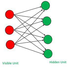
Restricted Boltzmann Machine Architecture

Example:

In this example, we will demonstrate the use of RBM features for digit classification using the MNIST (Modified National Institute of Standards and Technology) dataset, which consists of handwritten digits ranging from 0 to 9.

Steps for the usage of an RBM in combination with logistic regression for classification tasks are:

• Step 1: The very first step is to import the necessary libraries
  • BernoulliRBM from sklearn.neural_network
  • Pipeline from sklearn.pipeline
  • load_digits from sklearn.datasets
  • train_test_split from sklearn.model_selection
  • classification_report from sklearn.metrics 
• Step 2: load the MNIST data set
  • MNIST data set is been used with the help of the load_digits() function.
  • Separate input features and target variables.
  • Apply the min-max scaled to the datasets
• Step 3: Split the data into training and testing sets
  • train_test_split(): to split the loaded dataset into training and testing sets. 
• Step 4: Create an RBM model
  • creates an object of the BernoulliRBM class
• Step 5: Create a classifier
  • creates an object of the LogisticRegression class
• Step 6: Create a pipeline combining RBM and classifier
  •  creates a Pipeline object from sklearn.pipeline which combines the RBM and classifier together in a sequence
• Step 7: Train the model
  • trains the pipeline by calling the fit() method on the pipeline object
• Step 8: Make predictions on the test set
  • Use the trained pipeline to make predictions on the test set (X_test) by calling the predict method.
• Step 9: Evaluate the model
  • The code calculates and prints the classification report using the classification_report() function.

Python3

# Import necessary libraries
from sklearn.neural_network import BernoulliRBM
from sklearn.linear_model import LogisticRegression
from sklearn.pipeline import Pipeline
from sklearn.datasets import load_digits
from sklearn.preprocessing import minmax_scale, OneHotEncoder
from sklearn.model_selection import train_test_split
from sklearn.metrics import classification_report

# Load the MNIST dataset
digits = load_digits()

# Digits image
X = digits.data
# Digits
Y = digits.target

# Min-max scaling
X_scaled = minmax_scale(X, feature_range=(0, 1))

# Split the data into training and testing sets
X_train, X_test, y_train, y_test = train_test_split(X_scaled, Y,
                                                    test_size=0.2, random_state=42)

Epoch = 15
# Create an RBM model
rbm = BernoulliRBM(n_components=100, learning_rate=0.02, n_iter=Epoch,
                   random_state=42, verbose=True)

# Create a classifier
classifier = LogisticRegression(max_iter=500)

# Create a pipeline combining RBM and classifier
pipeline = Pipeline(steps=[('rbm', rbm), ('classifier', classifier)])

# Train the model
pipeline.fit(X_train, y_train)

# Make predictions on the test set
y_pred = pipeline.predict(X_test)

# Evaluate the model
print('\nClassification Report :\n',classification_report(y_test, y_pred))

Output:

[BernoulliRBM] Iteration 1, pseudo-likelihood = -26.07, time = 0.03s
[BernoulliRBM] Iteration 2, pseudo-likelihood = -25.78, time = 0.03s
[BernoulliRBM] Iteration 3, pseudo-likelihood = -25.69, time = 0.03s
[BernoulliRBM] Iteration 4, pseudo-likelihood = -25.56, time = 0.06s
[BernoulliRBM] Iteration 5, pseudo-likelihood = -25.77, time = 0.03s
[BernoulliRBM] Iteration 6, pseudo-likelihood = -25.55, time = 0.03s
[BernoulliRBM] Iteration 7, pseudo-likelihood = -25.62, time = 0.04s
[BernoulliRBM] Iteration 8, pseudo-likelihood = -25.38, time = 0.04s
[BernoulliRBM] Iteration 9, pseudo-likelihood = -24.95, time = 0.03s
[BernoulliRBM] Iteration 10, pseudo-likelihood = -24.67, time = 0.03s
[BernoulliRBM] Iteration 11, pseudo-likelihood = -23.88, time = 0.03s
[BernoulliRBM] Iteration 12, pseudo-likelihood = -23.51, time = 0.04s
[BernoulliRBM] Iteration 13, pseudo-likelihood = -22.78, time = 0.04s
[BernoulliRBM] Iteration 14, pseudo-likelihood = -22.45, time = 0.04s
[BernoulliRBM] Iteration 15, pseudo-likelihood = -21.96, time = 0.04s

Classification Report :
               precision    recall  f1-score   support

           0       0.91      0.94      0.93        33
           1       0.66      0.75      0.70        28
           2       0.72      0.85      0.78        33
           3       0.76      0.82      0.79        34
           4       0.94      1.00      0.97        46
           5       0.83      0.64      0.72        47
           6       0.97      0.94      0.96        35
           7       0.81      0.85      0.83        34
           8       0.78      0.47      0.58        30
           9       0.60      0.68      0.64        40

    accuracy                           0.80       360
   macro avg       0.80      0.79      0.79       360
weighted avg       0.80      0.80      0.79       360

Explanation:

The output of the code will display the classification report. In this report, there are 4 cols with the name precision, recall, and F1-score for each digit class, indicating the accuracy and reliability of the model’s predictions and the support value represents the number of samples for each class in the test set.

The model can achieve competitive performance in digit classification tasks by learning meaningful representations of the digit images using RBM features.

Applications of Restricted Boltzmann Machine

Restricted Boltzmann Machines (RBMs) have found numerous applications in various fields, some of which are:

• Collaborative filtering: RBMs are widely used in collaborative filtering for recommender systems. They learn to predict user preferences based on their past behavior and recommend items that are likely to be of interest to the user.
• Image and video processing: RBMs can be used for image and video processing tasks such as object recognition, image denoising, and image reconstruction. They can also be used for tasks such as video segmentation and tracking.
• Natural language processing: RBMs can be used for natural language processing tasks such as language modeling, text classification, and sentiment analysis. They can also be used for tasks such as speech recognition and speech synthesis.
• Bioinformatics: RBMs have found applications in bioinformatics for tasks such as protein structure prediction, gene expression analysis, and drug discovery.
• Financial modeling: RBMs can be used for financial modeling tasks such as predicting stock prices, risk analysis, and portfolio optimization.
• Anomaly detection: RBMs can be used for anomaly detection tasks such as fraud detection in financial transactions, network intrusion detection, and medical diagnosis.