Response of Second Order System

Control systems play a critical position in regulating and keeping the conduct of dynamic structures, making sure of balance and desired overall performance. One common form of machine encountered in the control idea is the second one-order system. The reaction of such structures is essential to understand for engineers and researchers operating in various fields. Now let’s move on to the concepts of pole and zero and the transient response to the second order system.

In contrast to the simplicity of first-order systems, second-order systems have many answers that need to be analyzed and explained. Changing first-order parameters only changes the response rate, while changing second-order parameters can change the response. For example, the second order may show similar behavior to the first order, or it may show temporary responses, either negative or weak, depending on the value of the product. In this article, we delve into the traits, analysis, and importance of the response of the second-order system on top of things theory.

What is a Second Order System?

A second-order system is a powerful framework portrayed by a second-degree transfer function in the Laplace domain. The general type of a second-order transfer function is addressed as:

G(s) = K / (s-a) (s-b)

where ,

K is the system gain,

s is the complex frequency variable, and

a and b are the system poles.

Derivation of Second Order System

To derive the transfer function of a 2nd-order system, remember an ordinary dynamic machine represented via a mass-spring-damper device. This system includes a mass m related to a spring with spring steady k and a damper with damping coefficient c. The input to the device is a force F(t), and the output is the displacement x(t) of the mass.

Applying Newton’s second law of motion to the mass yields the following second-order ordinary differential equation (ODE):

md²x / dt² + cdx/dt + kx = F(t)

here we are Taking the Laplace transform of both sides of the above equation, so we obtain:

ms² X(s) + csX(s) + KX(s) = F(s)

here the Laplace transforms of x(t) and F(t) are X(s) and F(s).

after this we will getting:

(ms² + cs + k) X(s) = F(s)

X(s)/F(s) = 1 / ms² + cs + k

This expression represents the transfer function G(s) of the second-order system, where:

K = 1/m

x = -c/2m + √c² – 4mk /2m

y = -c/2m – √c² -4mk / 2m

The poles x and y of the transfer function determine the nature of the system’s response: whether it is overdamped, underdamped, or critically damped.

Characteristic Equation of Second Order System

We know in the Second order System, the open loop transfer function is [Tex]\frac{\omega^2_n}{S(S+2\delta \omega_n)}[/Tex]

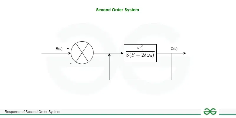
Second Order System

The Transfer function is given as

[Tex]\frac{C(s)}{R(s)}=\frac{G(s)}{1+G(s)}[/Tex]

now putting the value [Tex]\frac{\omega^2_n}{S(S+2\delta \omega_n)}[/Tex] in the transfer function

we get transfer function as

[Tex]\frac{C(s)}{R(s)}=\frac{\omega^2_n}{s^2+2\delta \omega_ns+\omega^2_n}[/Tex]

now the root characteristics can be found as

[Tex]s=-\delta \omega_n ± \omega_n \sqrt{\delta^2-1}[/Tex]

Now C(s) can be written as

C(s)=[Tex]C(s)=\frac{\omega^2_n}{s^2+2\delta \omega_ns+\omega^2_n}R(s)[/Tex]

Where,

C(s)=Laplace transform of output signal

R(s)=Laplace transform of Input signal

[Tex]\omega_n[/Tex]=natural frequency

[Tex]\delta [/Tex]=damping ratio

Characteristics of Second Order Systems

• Underdamped, Critically Damped, and Overdamped Response: The nature of the response relies upon at the places of the poles. If the poles are actual , the gadget is over-damped. If they’re complicated conjugates, the gadget is under damped. For poles at the real axis with multiplicity 2, the machine is seriously damped.
• Natural Frequency (ω_n ): The natural frequency is a essential function of second-order system. This shows the frequency at which the system would oscillate if there were no damping. It is denoted by means of ω_n and is related to the gap among the poles.
• Damping Ratio (ζ): The damping ratio is a degree of the level of damping within the system. It is denoted via ζ and impacts the kind of response. A better damping ratio effects in a slower response but with less oscillation.

Damping Ratio (ζ) = Exponential decay frequency / Natural frequency rad=second

• Peak Time, Rise Time, and Settling Time: These parameters are important in evaluating the overall performance of the gadget. The top time is the time taken to attain the height of the reaction, the upw thrust time is the time taken to reach from 10% to 90% of the final value, and the settling time is the time required for the reaction to stay inside a positive percent (commonly 5%) of the very last cost.

Step Response of Second Order System

The step response of a second-order system is a essential concept in control idea, offering perception into how the device behaves when subjected to a sudden alternate in its input signal, which include a step input. This reaction is characterized through various parameters and features, which are vital for analyzing and designing manage structures.

Derivation of Step Response of Second Order System

The step response of a second-order system can be derived from its transfer function G(s), which represents the connection among the Laplace remodel of the output and input signals.

G(s) = K / (s-a)(s-b)

where

K =system gain, and

a and b = system poles.

To obtain the step response, we first convert the step input signal into its Laplace transform. A unit step function

U(t) = 1/s . Thus, the Laplace transform of the step input signal r(t) is R(s)=1/s.

Next, we multiply the transfer function G(s) by the Laplace transform of the step input R(s) to obtain the Laplace transform of the output signal C(s):

C(s) =G(s).R(s) = 1 / (s-a)(s-b) .1/s

Performing partial fraction decomposition on C(s)

C(s) = A / (s-a) + B/ (s-b)

where

A and B are constants.

Transient Response Specification

The brief response of a 2nd-order machine is characterized by using numerous key parameters:

• Rise Time (t_r): The time taken for the reaction to rise from a certain low price (typically 10%) to a particular high cost (normally 90%).
• Peak Time (t_p): The time taken for the response to reach its peak value.

T_p = Л /ω_n √1- ζ²

• Settling Time (t_s): The time required for the reaction to settle inside a precise percentage (generally five%) of its final value and continue to be there.

T_s = 4 /ζω_n

• Overshoot (%OS): The maximum percentage by which the response overshoots its very last value.

%OS = e^{-(ζЛ √1 – ζ2)} ✕ 100

• Damping Ratio (ζ): A degree of the system’s damping, influencing the charge of decay of oscillations inside the response.

Damping Ratio (ζ) = Exponential decay frequency / Natural frequency

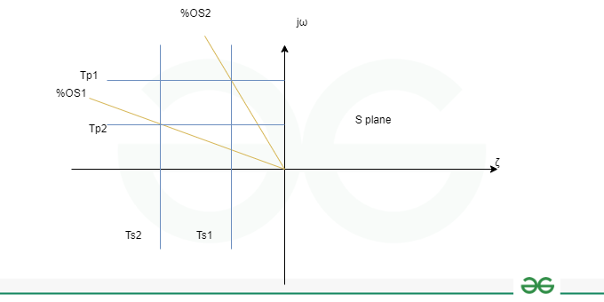
Transient Response Specification

Where, Lines of constant peak time, Tp, settling time, Ts, and percent overshoot, %OS are shown.

Ts2 < Ts1 ;Tp2 < Tp1; %OS1 < %OS2.

Types of Response of Second Order System

Some types of response of second order system are as follows:

• Purely oscillatory
• Underdamped Response
• Critically Damped Response
• Overdamped Response

Purely Oscillatory

For ζ=0

In this we have to substitute ζ=0 and R(s)=1/s

C(s)=[Tex]C(s)=\frac{1}{s}-\frac{1}{s+\omega_n}-\frac{\omega_n}{(s+\omega_n)^2}[/Tex]

Now doing inverse laplace transform we get as

[Tex] c(t) = (1 – \cos(\omega_nt))u(t) [/Tex]

Underdamped Response

For Underdamped system, 0< ζ < 1

Characterized through oscillations, the underdamped response is not unusual in systems in which the damping ratio (ζ) is less than 1. The reaction reaches the final value however famous a few overshoot.

Input and Response graph

For this transfer can be written as

[Tex]\frac{C(s)}{R(s)} = \frac{\omega^2_n}{(s + \delta \omega_n)^2 + \omega^2_n(1 – \delta^2)}[/Tex]

Now Substituting R(s)=1/s

[Tex]C(s) = \frac {\omega^2_n}{\left(\omega^2_n(s + \delta \omega_n)^2 + \omega^2_n(1 – \delta^2)\right)}\left(\frac{1}{s}\right) =\frac{\omega_n}{ s \left((s + \delta \omega_n)^2 + \omega^2_n(1 – \delta^2)\right)} [/Tex]

After solving using partial fraction we get as

[Tex]C(s) = \frac{1}{s} – \frac{(s + \delta \omega_n)}{(s + \delta \omega_n)^2 + \omega^2_d }-\frac{\delta}{\delta \sqrt{1 – \delta^2}} (\frac{\omega_d}{(s+\delta\omega_n)^2+\omega_d^2}) [/Tex]

After Applying laplace transform we get C(t) as

[Tex]c(t) = (1 – (\frac{e^{-\delta \omega_n t}}{\sqrt{1 – \delta^2}}) \sin(\omega_d t + \theta)u(t)[/Tex]

Critically Damped Response

For Critically Damped system, ζ = 1

The seriously damped response is the quickest response with out oscillations. It is carried out while the damping ratio (ζ) is identical to at least one. While it reaches the final price speedy, there may be no overshoot.

(a) Input (b) Response

[Tex]C(s) = \frac{\omega^2_n (s + \omega_n)^2}{(s+\omega_n)^2} = \frac{\omega_n^2}{s(s+\omega_n)^2} [/Tex]

After solving this using partial fraction we get equation as

[Tex]C(s)=\frac{1}{s}-\frac{1}{s+\omega_n}-\frac{\omega_n}{(s+\omega_n)^2}[/Tex]

Apply laplace transform as on both side we get equation as

[Tex]c(t) = (1 – e^{-\omega_nt} – \omega_nt e^{-\omega_nt})u(t) [/Tex]

Overdamped Response

For Overdamped system, ζ > 1

Overdamped structures showcase a slower response without a oscillations. This occurs whilst the damping ratio (ζ) is extra than 1. The response takes greater time to attain the very last fee however does so without overshooting.

(a) Input (b) Response

Transfer function can be written as

[Tex]\frac{C(s)}{R(s)} =\frac{ \omega^2_n}{(s + \delta \omega_n)^2 – \omega^2_n(\delta^2 – 1)} [/Tex]

R(s)=1/s

After solving equation using partial fraction we get as

[Tex]\begin{gathered} C(s)=\frac{1}{s}+\frac{1}{2\left(\delta+\sqrt{\delta^2-1}\right)\left(\sqrt{\delta^2-1}\right)}\left(\frac{1}{s+\delta \omega_n+\omega_n \sqrt{\delta^2-1}}\right) -\left(\frac{1}{2\left(\delta-\sqrt{\delta^2-1}\right)\left(\sqrt{\delta^2-1}\right)}\right)\left(\frac{1}{s+\delta \omega_n-\omega_n \sqrt{\delta^2-1}}\right) \end{gathered}[/Tex]

Applying inverse laplace transform we get as

[Tex]c(t)=\left(1+\left(\frac{1}{2\left(\delta+\sqrt{\delta^2-1}\right)\left(\sqrt{\delta^2-1}\right)}\right) e^{-\left(\delta \omega_n+\omega_n \sqrt{\delta^2-1}\right) t}-\left(\frac{1}{2\left(\delta-\sqrt{\delta^2-1}\right)\left(\sqrt{\delta^2-1}\right)}\right) e^{-\left(\delta \omega_n-\omega_n \sqrt{\delta^2-1}\right) t}\right) u(t)[/Tex]

Mathematical Formula for Response

The time-domain response of a second-order system can be expressed as a combination of exponential and trigonometric functions, depending on the type of response. The general structure is given by:

c(t) = c₁ e^s1t + c₂ e^s2t

where ,

s₁ and s₂ are the poles of the system and ,

c₁ and c₂ are constants.

Importance of Second Order System

Understanding second order response is important in many engineering programs:

• Control device design: Engineers use response capabilities to Construction meeting performance standards, minimal overshoot, rapid along with reaction time and stability.
• Filter Design: The second order system is common in filter designs. Response characteristics decide clear out conduct in phrases of frequency attenuation and segment shift.
• Mechanical Systems: In mechanical engineering, structures along with mass-spring-damping systems may be modeled 2nd-order. Analyzing their responses can assist expect and enhance their conduct.
• Circuits: Circuits, in particular those with RLC additives, may be modeled second-order. Analyzing the reaction helps design circuits with favored characteristics.

Conclusion

By deriving step responses from converting positions, engineers can apprehend how the system responds to adjustments in inputs, consisting of step inputs. Current response, such as rise time, peak time, settling time, overshoot, and damping ratio, affords many measurements to assess performance and balance. By examining step responses and periodic responses, engineers can layout and optimize systems to meet particular needs. These parameters manual the selection of manipulate techniques, modification of manage parameters, and evaluation of machine balance and robustness.

Additionally, trouble-fixing examples display the powerful use of assessment steps and updated answers in actual estate construction. Professionals can use this understanding to layout and analyze controls in a whole lot of industries, including aerospace, automotive, robotics and production. In reality, it’s miles the reaction of secondary system and the observe in their sustained response this is essential for engineers trying to create useful exceptional, stability and performance control to fulfill evolving needs. This is important within the modern-day global of generation and commercial enterprise.

Response of Second Order System – FAQs

What defines the nature of a second-order system’s response?

The position of the poles of a system (which may be real, complex or repetitive) determines its state (overdamped, underdamped or critically damped).

How does the damping ratio (ζ) affect the second order?

Damping ratio affects the damping level of the system, affecting overshoot, settling time and oscillation. Higher ζ leads to extreme behavior.

What is the natural frequency (ω_n) in the second-order system’s?

Natural frequency represents the frequency at which the system oscillates without damping. This will affects the performance of the system.

What are the three types of responses for second-order systems

Underdamping, critical damping and overdamping are three types of responses; consider this

How do engineers use response features in practical applications?

Design management, filter design, mechanical inspection etc. professionals in the fields. Use these components to create circuits for specific behaviors.