Control Systems – Polar Plots

Unlike the Bode plot in which both magnitude and phase angle are plotted separately in logarithmic graph paper. In Polar plot both magnitude and phase are plotted in the same plot in the Polar graph sheet. In the following article, we will discuss what is polar plot, Steps to draw polar plot, Polar plot of some standard Functions, and how to check the Stability of the system with a solved Example.

What is a Polar Plot?

Polar Graph Sheet

Polar plot is plot of magnitude |G(jω)H(jω)| versus phase angle ∠(G(jω)H(jω)) in polar coordinates and the value of frequency ie. ω is varied from 0 to ∞.

In polar plot magnitude of transfer function is plotted wrt to distance from origin and phase angle is plotted from positive real x-axis .Polar plot is used in Nyquist plot to determine the stability of closed loop control system from its open loop frequency response.

The transfer function G(jω)H(jω) can be represented as –

• Polar Form

G(jω)H(jω)=|G(jω)H(jω)| ∠ G(jω)H(jω)

where | G(jω)H(jω)| is magnitude represented as M(ω) of given transfer function and ∠ G(jω)H(jω) is phase angle represented as θ(ω)

• Rectangular Form

G(jω)H(jω) = Re[ G(jω)H(jω) ] +j Img[ G(jω)H(jω)]

In polar sheet graph magnitude of transfer function is represented by concentric circles and phase is represented by radial lines.In polar plot positive angle and negative angle both are represented in separate direction , in anti-clockwise direction positive angle is measured and in clockwise direction negative angle are measured taking 0 degree as reference point .

Angle Direction in Polar Plot

Steps To draw Polar Plots

Following are the steps to construct a polar plot of given transfer function G(s)H(s) –

Step 1: Determine the transfer function G(s)H(s) of given system.

Step 2: In place of s put s= jω in the transfer function to get G(jω)H(jω).

Step 3: Write the expression for magnitude |G(jω)H(jω)| and phase ∠ G(jω)H(jω) of transfer function.

Step 4: calculate the magnitude |G(jω)H(jω)|and phase ∠ G(jω)H(jω) of given transfer function by changing value of frequency ω from 0 to ∞ and construct the table as below.

Frequency (ω)	Magnitude ( |G(jω)H(jω)|) M(ω)	Phase Angle (∠ G(jω)H(jω)) θ(ω)
0	M(0)	θ(0)
ω1	M(ω1)	θ(ω1)
ω2	M(ω2)	θ(ω2)
ω3	M(ω3)	θ(ω3)
–	–	–
–	–	–
∞	M(∞)	θ(∞)

Step 5: Sketch the polar plot from the information from table .

Step 6: To determine the frequencies in which the plot crosses the real and imaginary axis , we rationalize the complex frequency transfer function G(jω)H(jω) by multiplying numerator and denominator of with complex conjugate of denominator factor of transfer function G(jω)H(jω). separate the real and imaginary part .

G(jω)H(jω) = Real [ G(jω)H(jω) ] +j Imaginary[ G(jω)H(jω)]

Step 7: The following cases can be followed :-

a)To determine the frequency at which polar plot intersect at real axis put imaginary part equals to 0

Img[G(jω)H(jω)]=0 , find ω

b) To find the frequency at which polar plot intersect at imaginary axis put real part equals to 0

Real [G(jω)H(jω)]=0 , find ω

Polar Plot of Some Standard Transfer Function

Following are the polar plot of some common standard function

Type 0

Order: 1

G(s)H(s) = 1 / (1+sT)

M(ω) = |G(jω)H(jω)| , θ(ω) = ∠ G(jω)H(jω)

ω = 0 , M = 1 , θ = 0⁰

ω = ∞ , M = 0 , θ = -90⁰

Type 0,Order 1

Order 2

G(s)H(s) =1 /(1 + sT1) (1 + sT2)

M(ω) = |G(jω)H(jω)| , θ(ω) = ∠ G(jω)H(jω)

ω = 0 , M = 1 , θ = 0⁰

ω = ∞ , M = 0 , θ = -180⁰

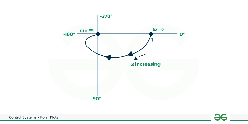
Type 0,Order 2

Type 1

Order: 1

G(s)H(s) = 1/s

M(ω) = |G(jω)H(jω)| , θ(ω) = ∠ G(jω)H(jω)

ω = 0 , M = ∞ , θ = -90⁰

ω = ∞ , M = 0 , θ = -90⁰

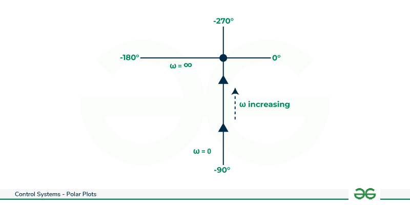
Type 1,Order1

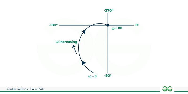
Order: 2

G(s)H(s) = 1/s(1 + sT)

M(ω) = |G(jω)H(jω)| , θ(ω) = ∠ G(jω)H(jω)

ω = 0 , M = ∞ , θ = -90⁰

ω = ∞ , M = 0 , θ = -180⁰

Type1,Order: 2

Order: 3

G(s)H(s) = 1/s(1 + sT1) (1 + sT2)

M(ω) = |G(jω)H(jω)| , θ(ω) = ∠ G(jω)H(jω)

ω = 0 , M = ∞ , θ = -90⁰

ω = ∞ , M = 0 , θ = -270⁰

Type1,Order 3

Type 2

Order: 4

G(s)H(s) = 1/s2(1 + sT1) (1 + sT2)

M(ω) = |G(jω)H(jω)| , θ(ω) = ∠ G(jω)H(jω)

ω = 0 , M = ∞ , θ = -180⁰

ω = ∞ , M = 0 , θ = 90⁰

Type 2 ,order 4

To Check the Stability of System from Polar Plot

To check the stability of system from Polar Plot we first need to determine Gain Margin (GM) ,Phase Margin (PM) , Gain Crossover Frequency (ω_GC) and Phase Cross over Frequency (ω_PC) of system .

Phase Cross Over Frequency (ω_PC)

It is the frequency at which phase angle ∠ G(jω)H(jω) of open loop transfer function G(jω)H(jω) becomes -180⁰ .

[∠ G(jω)H(jω) ]ω=ω_ωPC = -180⁰

Gain Cross Over Frequency (ω_GC)

It is the frequency at which magnitude |G(jω)H(jω)| of open loop transfer function G(jω)H(jω) becomes unity.

[ |G(jω)H(jω)| ] ω=ω_GC =1

Gain Margin (GM)

It is the factor or amount of gain required to bring the system on the verge of instability or to make system marginal stable.

It can also be defined as the reciprocal of the magnitude of open loop transfer function at phase cross over frequency ω_PC.

GM = 1 / a = 1 / |G(jω_PC)H(jω_PC)|

where ∠ G(jω_PC)H(jω_PC) = -180⁰

GM (in db) = 20 log ₁₀(GM)

0 < a < 1	GM (in db) > 0
a = 1	GM (in db) = 0
a > 1	GM (in db) < 0

Phase Margin (PM)

It is the amount of phase lag that can be introduced into the system at the gain cross over frequency ω_GC to derive the system to the verge of instability . It is expressed as –

PM = 180⁰ + ∠ G(jω_GC)H(jω_GC)

where |G(jω_GC)H(jω_GC)| = 1

Plot Representing Gain Cross Over and Phase Cross Over Frequency

Stability Determination from Polar Plot

Stability of system depends on its Gain Cross Over Frequency (ω_GC ), Phase Cross Over Frequency (ω_PC) , Gain Margin (GM) and Phase Margin (PM) .Following tables tells us how to determine stability –

ωPC > ωGC	GM >0 , PM >0	System is Stable
ωPC = ωGC	GM = 0 , PM = 0	System is Marginally Stable
ωPC < ωGC	GM < 0 , PM < 0	System is Unstable

Effects of adding Poles and zeroes in Polar Plots

Following are the effects of adding zeroes and poles :-

1. Addition of non-zero pole to a transfer function results in further rotation of the polar plot through an angle of -90⁰ as ω→∞
2. Addition of pole at the origin to a transfer function rotates the polar plot at 0 and infinite frequencies by a further angle of -90⁰
3. The effect of addition of a zero to a transfer function is to rotates the high frequency portion of the polar plot by 90⁰ in counter – clockwise direction.

Solved Example of Polar Plot

ques :- Sketch the polar plot of G(s)H(s) = 1/s(1+s)

Step 1: Determine Transfer function.

G(s)H(s) = 1/s(1+s)

Step 2: Put s=jω

G(ω)H(ω) = 1/ω(1+jω)

Step 3: Find magnitude and phase angle

M(ω) = |G(jω)H(jω)| = 1/ω(1+ω²)^1/2

θ(ω)= ∠ G(jω)H(jω) = -90⁰-tan^-1(ω)

Step 4: construct a table as below :

Frequency (ω)	Magnitude ( |G(jω)H(jω)|) M(ω)	Phase Angle (∠ G(jω)H(jω)) θ(ω)
0	∞	-900
1	0.7	-1350
2	0.22	-1530
5	0.039	-1690
–	–	–
∞	0	-1800

Step 5: Sketch the Polar Plot from above information

Polar Plot (solved)

Advantages and Disadvantage of Polar Plots

Following are some of the advantage and disadvantage of Polar Plots :-

Advantages of Polar Plots

• It gives the frequency response characteristic of system over the entire frequency range in a single plot.
• Easy to find the stability of system.
• Easy to find gain margin and phase margin directly from graph .

Disadvantage of Polar Plots

• It does not give information about contribution of each individual factor of open loop transfer function.
• Since polar plot is applicable for linear time invariant system so we can not do analysis in nonlinear system .
• we can not be able to analyze time domain characteristic such as rise time , peak time , max overshoot etc.

Application of Polar Plot

Following are some of the application of Polar Plot :-

• Used in Nyquist stability criteria
• Used to find Gain and Phase Margin
• Used to find Resonance Frequency
• Used to find Frequency Response of System

Conclusion

Polar Plot helps to understand behaviour of system and helps to analyze how system reacts in different frequency . It helps to find the stability of system . Through Polar plot we are able to easily find out the gain and phase margin of the system and the gain cross over and phase cross over frequency . we can also keep an eye on the performance of system through polar plot and also able to find out what should be done to make system stable and unstable .

FAQs on Polar Plots

Q1. What is the condition of stability for locus in Polar Plot ?

If critical Point (-1+0j) is enclosed by locus of Polar Plot system is unstable and if it is not enclosed than system is stable.

Q2. What is difference between Polar Plot and Nyquist Plot ?

In Nyquist Plot the frequency range varies from -∞ to +∞ where as in Polar Plot frequency range varies from 0 to +∞.

Q3. What are the Application of Polar Plot ?

The main application of Polar Plot is that it is used to apply Nyquist Stability criteria to find stability of system.

Q4. How is magnitude and phase angle measured in Polar Plot ?

In Polar Plot the magnitude of transfer function is plotted as distance from origin and phase angle is is measured from positive real axis .