Regression Tree with Simulated Data – rpart package

Regression trees are a type of machine-learning algorithm that is used for predicting continuous outcomes. They are a popular choice for modeling complex relationships between predictors and outcomes, as they are able to capture nonlinearities and interactions that may be missed by more traditional linear models. One popular implementation of regression trees in R Programming Language is the rpart package, which provides an easy-to-use interface for building and visualizing regression trees.

In this article, we will walk through an example of how to use the rpart package to build a regression tree using simulated data. We will begin by discussing what regression trees are and how they work, before moving on to a step-by-step guide on building a regression tree using rpart.

What are Regression Trees?

Regression trees are a type of decision tree that is used for predicting continuous outcomes. They work by partitioning the predictor space into a series of subspaces and then fitting a simple model (usually a mean or a constant) to the data within each subspace. The tree is built by recursively splitting the predictor space into smaller and smaller subspaces until some stopping criterion is met (e.g., a minimum number of observations in each subspace).

Each split in the tree is chosen to minimize the residual sum of squares (RSS) between the predicted values and the actual values of the outcome variable. This is done by evaluating all possible splits of the predictor space at each step and choosing the split that results in the largest reduction in RSS.

Once the tree is built, it can be used to predict the outcome variable for new observations by traversing the tree from the root node to a leaf node and returning the mean or constant value associated with that leaf node.

Building a Regression Tree with rpart

R

library(rpart)

# Simulate data
set.seed(123)
n <- 100
x1 <- runif(n)
x2 <- runif(n)
y <- ifelse(x1 + x2 > 1,
            x1 - x2, x1 + x2) + rnorm(n,
                                      sd = 0.2)
data <- data.frame(x1 = x1,
                   x2 = x2, y = y)

# Build regression tree
tree <- rpart(y ~ x1 + x2,
              data = data)

# Plot tree
plot(tree, main = "Regression Tree")

# Predict values for new data
new_data <- data.frame(x1 = seq(0, 1, 0.1),
                       x2 = seq(0, 1, 0.1))
pred <- predict(tree, new_data)
plot(y ~ x1 + x2, data = data,
     main = "Predictions from Regression Tree")
points(x = new_data$x1, y = pred,
       pch = 20, col = "red")

Output for x1:

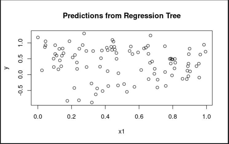
Scatter plot for x1 using rpart package

Output for x2:

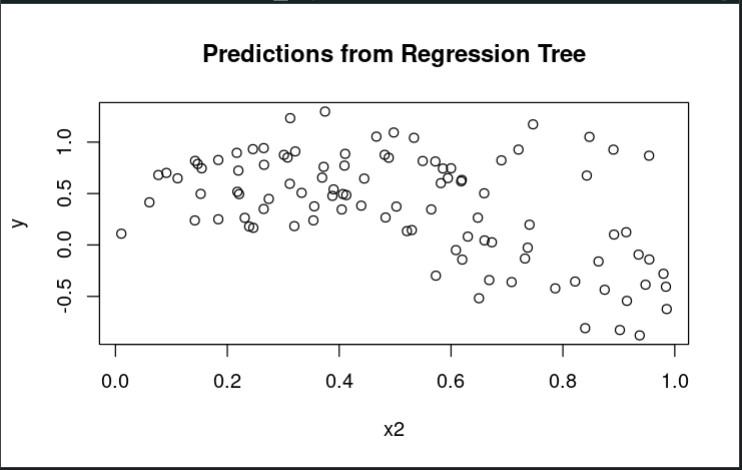
Scatter plot for x2 using rpart package

To illustrate how to build a regression tree using rpart, we will simulate some data and then fit a tree to the data. We will use the following code to generate our simulated data:

R

# Set the seed for reproducibility
set.seed(123)

# Define the number of observations to generate
n <- 1000

# Generate three predictor variables
# from a uniform distribution
x1 <- runif(n)
x2 <- runif(n)
x3 <- runif(n)

# Generate the response variable as a function of the
# predictor variables plus some random noise
y <- 2*x1 + 3*x2^2 + 0.5*sin(2*pi*x3) + rnorm(n,
                                              mean = 0,
                                              sd = 1)

# Create a data frame containing the
# predictor variables and the response variable
sim_data <- data.frame(x1 = x1, x2 = x2,
                       x3 = x3, y = y)

In this code, we generate three predictor variables (x1, x2, and x3) and one outcome variable (y). The relationship between the predictors and the outcome is intentionally complex, with x1 and x2 having a quadratic effect and x3 having a sinusoidal effect.

We can visualize the relationship between the predictors and the outcome using the following code:

R

# Load the ggplot2 package for data visualization
library(ggplot2)

# Create a scatter plot of x1
# against y with a linear regression line
ggplot(sim_data, aes(x = x1, y = y)) +
  geom_point() +
  geom_smooth(method = "lm",
              formula = "y ~ x1", se = FALSE)

# Create a scatter plot of x2
# against y with a quadratic regression line
ggplot(sim_data, aes(x = x2, y = y)) +
  geom_point() +
  geom_smooth(method = "lm",
              formula = "y ~ x2", se = FALSE)

# Create a scatter plot of x3
# against y with a sinusoidal regression line
ggplot(sim_data, aes(x = x3, y = y)) +
  geom_point() +
  geom_smooth(method = "lm",
              formula = "y ~ x3", se = FALSE)

Output:

Scatter plot for x₁:

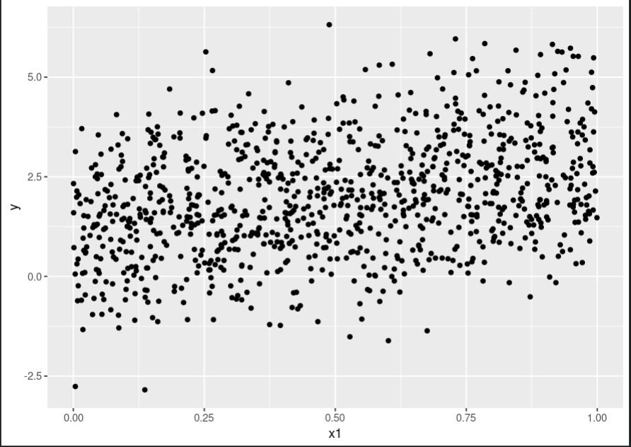
Scatter plot for x1 using rpart package

Scatter plot for x₂:

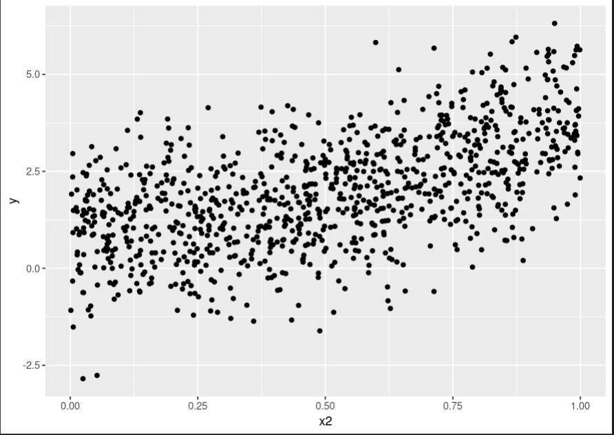
Scatter plot for x2 using rpart package

Scatter plot for x₃:

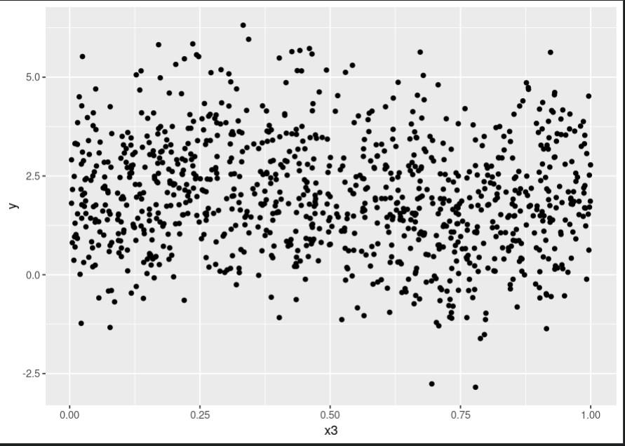
Scatter plot for x3 using rpart package

This code produces three plots, one for each predictor, showing the relationship between that predictor and the outcome variable. As we can see, the relationship is quite complex and nonlinear.

To build our regression tree, we will use the rpart() function from the rpart package. The `rpart` function requires three arguments: the formula specifying the outcome variable and predictor variables, the data frame containing the data, and any additional control options. We will use the following code to build our tree:

R

library(rpart)
tree <- rpart(y ~ x1 + x2 + x3,
              data = sim_data,
              control = rpart.control(minsplit = 10,
                                      cp = 0.01))

In this code, we specify the formula y ~ x1 + x2 + x3 to indicate that we want to predict y using x1, x2, and x3. We pass in the sim_data data frame as the data argument, and set the minsplit argument to 10 and the cp (complexity parameter) argument to 0.01 to control the complexity of the tree.

We can visualize the resulting tree using the plot() function:

R

plot(tree)
text(tree)

Output:

This code produces a plot of the tree, with each node labeled with the splitting variable and value, as well as the mean value of y for the observations in that node. The text() function adds the numerical values to the plot.

We can see that the tree has split the predictor space into multiple subspaces, with each subspace associated with a particular value of y. The splits are chosen to maximize the reduction in RSS, subject to the minimum split size and complexity parameter constraints.

We can use the predict() function to make predictions for new observations:

R

new_data <- data.frame(x1 = 0.5,
                       x2 = 0.5,
                       x3 = 0.5)
predict(tree, new_data)

Output:

       1 
1.925488 

In this code, we create a new data frame containing predictor values for a new observation and then use the predict() function with the tree object and new_data as arguments to predict the value of y for that observation. The predicted value is returned as a single number.

Conclusion:

Regression trees are a powerful tool for modeling complex relationships between predictors and outcomes. In this article, we demonstrated how to use the rpart package in R to build a regression tree using simulated data. We discussed the underlying principles of regression trees and provided a step-by-step guide to building and visualizing a tree using rpart. With this knowledge, you should be able to use regression trees to model your own data and make predictions for new observations.