Data analysis using Python’s Pandas library is a powerful process, and its efficiency can be enhanced with specific tricks and techniques. These Python tips will make our code concise, readable, and efficient. The adaptability of Pandas makes it an efficient tool for working with structured data. Whether you are a beginner or an experienced data scientist, mastering these Python tips can help you enhance your efficiency in data analysis tasks.
.png)
Pandas tips for Data Analysis
In this article we will explore about What are the various 10 python panads tips to make data analysis faster and that helps us to make our work more easier.
Use Vectorized Operation
Pandas is a library in Python supports vectorized operations. We can efficiently utilize these operations whenever possible instead of iterating through rows. For example, instead of using a for loop to perform calculations on each row, we can apply operations directly to entire columns.
Iterative Approach:
Python3
import pandas as pd
data = {'old_column': [1, 2, 3, 4, 5]}
df = pd.DataFrame(data)
for index, row in df.iterrows():
df.at[index, 'new_column'] = row['old_column'] * 2
print("DataFrame after looping through rows:")
print(df)
|
Output:
DataFrame after looping through rows:
   old_column  new_column
0           1         2.0
1           2         4.0
2           3         6.0
3           4         8.0
4           5        10.0
Vectorized Approach:
When a vectorized approach is used for the above operation, the entire calculation is applied at once. The entire old column values are multiplied by 2 and the result is assigned to the new column (‘new_column’).
Python3
import pandas as pd
data = {'old_column': [1, 2, 3, 4, 5]}
df = pd.DataFrame(data)
df['new_column'] = df['old_column'] * 2
print("\nDataFrame after using vectorized operations:")
print(df)
|
Output:
DataFrame after using vectorized operations:
   old_column  new_column
0           1           2
1           2           4
2           3           6
3           4           8
4           5          10
Optimize Memory Usage
We can optimize memory usage by using appropriate data types for columns. This will significantly reduce the amount of memory consumed by a dataframe. Let’s discuss this with an example.
Consider we have a dataframe with a column named ‘column’ with floating-point numbers. By default, Pandas uses float64 data type to represent these numbers. However, for our data the precision of float32 is sufficient. In such cases, we can reduce the memory footprint by converting the column to float32.
Python3
import pandas as pd
data = {'column': [1.0, 2.5, 3.8, 4.2, 5.6]}
df = pd.DataFrame(data)
print("Original DataFrame:")
print(df)
print(df.info())
print("\nMemory usage before optimization:")
print(df.memory_usage())
|
Output:
Original DataFrame:
   column
0     1.0
1     2.5
2     3.8
3     4.2
4     5.6
<class 'pandas.core.frame.DataFrame'>
RangeIndex: 5 entries, 0 to 4
Data columns (total 1 columns):
 #   Column  Non-Null Count  Dtype
---  ------  --------------  -----
 0   column  5 non-null      float64
dtypes: float64(1)
memory usage: 168.0 bytes
None
Memory usage before optimization:
Index     128
column     40
dtype: int64
The above output shows that the ‘column’ is of type float64, and the memory usage is 7.9 KB. Now, let’s optimize the memory usage by converting the column to float32:
Python3
df['column'] = df['column'].astype('float32')
print("\nDataFrame after optimizing memory usage:")
print(df)
print(df.info())
print("\nMemory usage after optimization:")
print(df.memory_usage())
|
Output:
DataFrame after optimizing memory usage:
   column
0     1.0
1     2.5
2     3.8
3     4.2
4     5.6
<class 'pandas.core.frame.DataFrame'>
RangeIndex: 5 entries, 0 to 4
Data columns (total 1 columns):
 #   Column  Non-Null Count  Dtype
---  ------  --------------  -----
 0   column  5 non-null      float32
dtypes: float32(1)
memory usage: 148.0 bytes
None
Memory usage after optimization:
Index     128
column     20
dtype: int64
After converting the column to float32, the memory usage was reduced to 148 B. This demonstrates a significant reduction in memory consumption while still maintaining the required level of precision.
Method Chaining
Method chaining is a programming pattern in Pandas that allows us to apply a sequence of operations to a dataframe in a single line of code.
Example: In the below example, We are performing the operations like dropping nan values, renaming the column, grouping and resetting the index as separate steps. Each operation creates an intermediate dataframe which is modified in the next step. This leads to increased memory usage.
Python3
data = {
'column1': [1, 2, None, 4, 5],
'column2': ['A', 'B', 'C', 'D', 'E']
}
df = pd.DataFrame(data)
df = df.dropna(subset=['column1'])
df = df.rename(columns={'column2': 'new_column'})
df = df.reset_index(drop=True)
print("DataFrame without method chaining:")
print(df)
|
Output:
DataFrame without method chaining:
   column1 new_column
0      1.0          A
1      2.0          B
2      4.0          D
3      5.0          E
Using the method chaining method, each operation is applied directly to the dataframe. This reduces the memory usage and enhances the conciseness. To ensure correct method chaining use parenthesis.
Python3
df = (pd.DataFrame(data)
.dropna(subset=['column1'])
.rename(columns={'column2': 'new_column'})
.reset_index(drop=True))
print("\nDataFrame with method chaining:")
print(df)
|
Output:
DataFrame with method chaining:
   column1 new_column
0      1.0          A
1      2.0          B
2      4.0          D
3      5.0          E
Use GroupBy Aggregations
GroupBy aggregations in Pandas is an efficient way to perform operations on subsets of data based on specific criteria rather than iterating through rows manually.
Example: Consider the following example of calculating the average value of each category.
Python3
import pandas as pd
data = {'Category': ['A', 'B', 'A', 'B', 'A', 'B'],
'Value': [10, 20, 15, 25, 12, 18]}
df = pd.DataFrame(data)
categories = df['Category'].unique()
for category in categories:
avg_value = df[df['Category'] == category]['Value'].mean()
print(f'Average Value for Category {category}: {avg_value}')
|
In the above code, the number of categories are first retrieved. The average of each category is calculated by using for loop on each category.
Output:
Average Value for Category A: 12.333333333333334
Average Value for Category B: 21.0
Using Group by:
Instead of iterating through rows to perform aggregations, we can use the groupby function to group data and apply aggregate functions efficiently.
Python3
import pandas as pd
data = {'Category': ['A', 'B', 'A', 'B', 'A', 'B'],
'Value': [10, 20, 15, 25, 12, 18]}
df = pd.DataFrame(data)
result = df.groupby('Category')['Value'].mean()
print(result)
|
Here, we group the DataFrame df by the ‘Category’ column using groupby (‘Category’). Then, we apply the mean() aggregate function to the ‘Value’ column within each group. The result is a Series with the average value for each category.
Output:
Category
A    12.333333
B    21.000000
Name: Value, dtype: float64
Using describe() and Percentile
In data analysis, the describe and percentile functions help to understand the distribution and summary statistics of a dataset. Describe function gives us the statistical properties like count, mean, standard deviation, min, max, etc for the numerical columns. Percentile divides the dataset into specific percentage intervals like 20%, 40%, 60%, and 80%. In some scenarios, our analysis needs these percentile values to be included in the summary given by the describe function. In such cases, we can use percentiles within the describe function.
Example: In the below code, we are getting the summary using describe function and then calculating the required percentiles.
Python3
import pandas as pd
data = {'Value': [10, 15, 20, 25, 30, 35, 40, 45, 50]}
df = pd.DataFrame(data)
summary_stats = df['Value'].describe()
print(summary_stats)
percentile_25 = df['Value'].quantile(0.25)
percentile_50 = df['Value'].quantile(0.50)
percentile_75 = df['Value'].quantile(0.75)
print(f'25th Percentile: {percentile_25}')
print(f'50th Percentile (Median): {percentile_50}')
print(f'75th Percentile: {percentile_75}')
|
Output:
count     9.000000
mean     30.000000
std      13.693064
min      10.000000
25%      20.000000
50%      30.000000
75%      40.000000
max      50.000000
Name: Value, dtype: float64
25th Percentile: 20.0
50th Percentile (Median): 30.0
75th Percentile: 40.0
Combining describe and percentile: We can efficiently summarize the code by including percentiles in the describe function. It gives the percentile values along with the describe function’s summary. Let’s see the code.
Python3
import pandas as pd
data = {'Value': [10, 15, 20, 25, 30, 35, 40, 45, 50]}
df = pd.DataFrame(data)
summary_stats = df['Value'].describe(percentiles=[0.25, 0.5, 0.75])
print(summary_stats)
|
Output:
count     9.000000
mean     30.000000
std      13.693064
min      10.000000
25%      20.000000
50%      30.000000
75%      40.000000
max      50.000000
Name: Value, dtype: float64
Leverage the Power of pd.cut and pd.qcut
The pd.cut and pd.qcut functions in Pandas are used for binning numerical data into discrete intervals or quantiles, respectively. These functions are useful for various data analysis and machine learning tasks. Let’s discuss this in detail.
1. pd.cut:
The pd.cut function is used for binning continuous data into discrete intervals (bins). Further, this can be used to convert continuous variables to categorical variables. We can analyze various patterns from this.
Example: In this example, the numerical column ‘Values’ is divided into three bins (Low, Medium, High) using pd.cut. Each value is assigned to the appropriate bin based on the specified intervals.
Python3
import pandas as pd
data = {'Values': [5, 12, 18, 25, 32, 40, 50, 60]}
df = pd.DataFrame(data)
bins = [0, 20, 40, 60]
labels = ['Low', 'Medium', 'High']
df['Binned_Values'] = pd.cut(df['Values'], bins=bins, labels=labels)
print(df)
|
Output:
  Values Binned_Values
0       5           Low
1      12           Low
2      18           Low
3      25        Medium
4      32        Medium
5      40        Medium
6      50          High
7      60          High
2. pd.qcut:
The pd.qcut function does bin based on quantiles. This is used when we need to bin similar distribution values together. It divides the data into discrete intervals based on the given quantiles. This is particularly useful when you want to ensure that each bin contains a similar distribution of values.
Example: In this example, the numerical column ‘Values’ is divided into four quantile-based bins (Q1, Q2, Q3, Q4) using pd.qcut.
Python3
data = {'Values': [5, 12, 18, 25, 32, 40, 50, 60]}
df = pd.DataFrame(data)
df['Quantile_Binned'] = pd.qcut(df['Values'], q=[0, 0.25, 0.5, 0.75, 1], labels=['Q1', 'Q2', 'Q3', 'Q4'])
print(df)
|
Output:
Values Quantile_Binned
0       5              Q1
1      12              Q1
2      18              Q2
3      25              Q2
4      32              Q3
5      40              Q3
6      50              Q4
7      60              Q4
Optimize DataFrame Merging
Merge function in Pandas is used to combine two or more DataFrames based on a common column or index. While merging, the dataframes can be optimized by specifying on and how parameters to improve the performance. Let’s discuss with an example:
1.on Parameter:
The on parameter specifies the column or index on which the merging should occur. If the columns to be merged, have the same name in both DataFrames, we can use this parameter to specify the common column explicitly.
Example: In this example, the on=’ID’ parameter explicitly specifies that the merging should occur based on the ‘ID’ column.
Python3
import pandas as pd
df1 = pd.DataFrame({'ID': [1, 2, 3], 'Value1': ['A', 'B', 'C']})
df2 = pd.DataFrame({'ID': [1, 2, 3], 'Value2': ['X', 'Y', 'Z']})
merged_df = pd.merge(df1, df2, on='ID')
print(merged_df)
|
Output:
   ID Value1 Value2
0   1      A      X
1   2      B      Y
2   3      C      Z
2. how Parameter:
The how parameter determines the type of merge to be performed. ‘left’, ‘right’, ‘outer’, and ‘inner’ are some common options. We can specify this term explicitly to perform the desired type of merging.
Example:
Python3
import pandas as pd
df1 = pd.DataFrame({'ID': [1, 2, 3], 'Value1': ['A', 'B', 'C']})
df2 = pd.DataFrame({'ID': [2, 3, 4], 'Value2': ['X', 'Y', 'Z']})
merged_df_inner = pd.merge(df1, df2, on='ID', how='inner')
merged_df_outer = pd.merge(df1, df2, on='ID', how='outer')
print("Inner Merge:")
print(merged_df_inner)
print("\nOuter Merge:")
print(merged_df_outer)
|
Output: In the ‘inner’ merge, only the common IDs present in both DataFrames are retained. In the ‘outer’ merge, all IDs from both DataFrames are retained, filling in missing values with NaN when necessary.
Inner Merge:
   ID Value1 Value2
0   2      B      X
1   3      C      Y
Outer Merge:
   ID Value1 Value2
0   1      A    NaN
1   2      B      X
2   3      C      Y
3   4    NaN      Z
Use isin for Filtering
The isin method in Pandas is used to filer a DataFrame based on multiple values. This method is useful when we want to select rows where a specific column matches any of the given values. Let’s discuss with an example.
1. Without isin Method:
Example: In this example, we have a DataFrame df with columns ‘ID’, ‘Category’, and ‘Value’. We want to filter rows where the ‘Category’ column matches any value in the list [‘A’, ‘B’].
Python3
import pandas as pd
data = {'ID': [1, 2, 3, 4, 5],
'Category': ['A', 'B', 'A', 'C', 'B'],
'Value': [10, 20, 15, 25, 30]}
df = pd.DataFrame(data)
categories_to_filter = ['A', 'B']
filtered_df = df[df['Category'].apply(lambda x: x in categories_to_filter)]
print("Filtered DataFrame (Without isin):")
print(filtered_df)
|
Output:
Filtered DataFrame (Without isin):
   ID Category  Value
0   1        A     10
1   2        B     20
2   3        A     15
4   5        B     30
Take Advantage of .loc for Conditional Updates:
We can use the .loc for conditional updates of DataFrame values. This method is more efficient than using loops. The .loc accessor allows us to select and modify data based on conditions without the need for iteration over rows. Let’s discuss this with an example.
With .loc:
Python3
import pandas as pd
data = {'ID': [1, 2, 3, 4, 5],
'Category': ['A', 'B', 'A', 'C', 'B'],
'Value': [10, 20, 15, 25, 30]}
df = pd.DataFrame(data)
df.loc[df['Value'] > 20, 'Category'] = 'High'
df.loc[df['Value'] <= 20, 'Category'] = 'Low'
print("\nUpdated DataFrame (With .loc):")
print(df)
|
Output:
Updated DataFrame (With .loc):
   ID Category  Value
0   1      Low     10
1   2      Low     20
2   3      Low     15
3   4     High     25
4   5     High     30
Profile Code with ydata_profiling
ydata_profiling is an open-source Python library that provides an easy way to create profiling reports for Pandas DataFrames. These reports offer insights into the structure, statistics, and issues within the dataset. Profiling is an important step in the data analysis process, helping to identify bottlenecks, missing values, duplicates, and other characteristics that require attention or optimization. Using ydata_profiling we can profile our data, especially when dealing with large and complex datasets. It provides a comprehensive set of visualizations and insights that can guide our data analysis and preprocessing efforts.
Here’s a detailed explanation of how to use ydata_profiling to profile your code:
1. Installation: Before using ydata_profiling, you need to install it. You can install it using the following command:
pip install ydata-profiling
2. Importing and Generating Profile Report:
Python3
import pandas as pd
import ydata_profiling
data = {'ID': [1, 2, 3, 4, 5],
'Category': ['A', 'B', 'A', 'C', 'B'],
'Value': [10, 20, 15, 25, 30]}
df = pd.DataFrame(data)
profile = ydata_profiling.ProfileReport(df)
profile.to_file("data_profiling_report.html")
profile.to_widgets()
|
Output:
Updated DataFrame (With .loc):
   ID Category  Value
0   1      Low     10
1   2      Low     20
2   3      Low     15
3   4     High     25
4   5     High     30
Steps performed in the above code:
- Import the necessary libraries: pandas, pandas_profiling.
- Create a sample DataFrame (df in this case).
- Use pandas_profiling.ProfileReport() to generate a profiling report for the DataFrame.
- Optionally, save the report to an HTML file using to_file.
- Display the report using to_widgets.
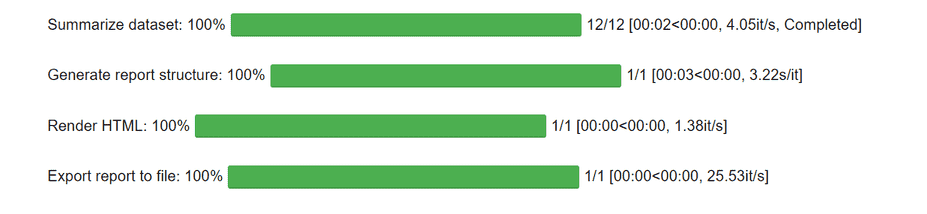
profile processing by ydata_profiling
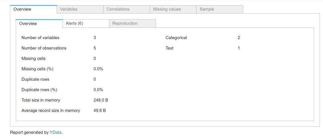
Report generated by ydata_profiling
3. Interpreting the Report:
The profiling report includes various sections:
- Overview: General information about the DataFrame, including the number of variables, observations, and memory usage.
- Variables: Detailed information about each variable, including type, unique values, missing values, and a histogram.
- Interactions: Correlation matrix and scatter plots for numeric variables.
- Missing Values: Heatmap showing the locations of missing values in the DataFrame.
- Sample: A sample of rows from the DataFrame.
- Warnings: Potential issues and warnings based on the analysis.
- Histograms: Histograms for numeric variables.
- Correlations: Correlation matrix and heatmap.
- Missing Values Dendrogram: Dendrogram visualizing missing value patterns.
- Text Reports: Text-based summaries for each variable.
Conclusion
In conclusion, using advanced techniques and tricks in Python’s Pandas library can significantly enhance the efficiency and effectiveness of data analysis. These ten tips, ranging from utilizing vectorized operations to profiling code with pandas_profiling, offer ways to streamline the workflow, improve code readability, and optimize performance.
10 Python Pandas tips to make data analysis faster- FAQ
1. Why should we prefer vectorized operations in Pandas for data analysis?
Pandas’ library in Python supports vectorized operations. We can efficiently utilize these operations whenever possible instead of iterating through rows. For example, instead of using a for loop to perform calculations on each row, we can apply operations directly to entire columns.
2. How can I optimize memory usage in pandas dataframe?
We can optimize memory usage by using appropriate data types for columns. This will significantly reduce the amount of memory consumed by a dataframe. If a data requires 32 bits, reduce the allotted space from 64 bits to 32 bits. Choosing the right memory space optimizes the memory usage.
3. What is method chaining in Pandas, and how does it enhance data analysis code?
Method chaining is a programming pattern in Pandas that allows us to apply a sequence of operations to a dataframe in a single line of code. It enhances code conciseness, and increases performance by avoiding intermediate dataframes.
4. How can I efficiently perform groupby aggregations in Pandas for data analysis?
GroupBy aggregations in Pandas is an efficient way to perform operations on subsets of data based on specific criteria rather than iterating through rows manually.
Share your thoughts in the comments
Please Login to comment...