Parallel Algorithm Models in Parallel Computing

Parallel Computing is defined as the process of distributing a larger task into a small number of independent tasks and then solving them using multiple processing elements simultaneously. Parallel computing is more efficient than the serial approach as it requires less computation time.  

Parallel Algorithm Models

The need for a parallel algorithm model arises in order to understand the strategy that is used for the partitioning of data and the ways in which these data are being processed. Therefore every model being used provides proper structuring based on two techniques. They are as follows:

1. Selection of proper partitioning and mapping techniques.

2. Proper use of strategy in order to reduce the interaction.

Types of Parallel Models

1. The Data-Parallel Model

The data-parallel model algorithm is one of the simplest models of all other parallel algorithm models. In this model, the tasks that need to be carried out are identified first and then mapped to the processes. This mapping of tasks onto the processes is being done statically or semi-statically. In this model, the task that is being performed by every process is the same or identical but the data on which these operations or tasks are performed is different.

The problem to be solved is divided into a number of tasks on the basis of data partitioning. Here data partitioning is being used because all the operations performed by each process are similar and proper uniform partitioning of data followed by static mapping assures the proper load balancing. 

Example: Dense Matrix Multiplication

Dense Matrix  Multiplication

In the above example of dense matrix multiplication, the instruction stream is being divided into the available number of processors. Each processor computes the data stream it is allocated with and accesses the memory unit for read and write operation. As shown in the above figure, the data stream 1 is allocated to processor 1, once it computes the calculation the result is being stored in the memory unit.

2. The Task Graph Model

The task dependency graph is being used by the parallel algorithms for describing the computations it performs. Therefore, the use of interrelationships among the tasks in the task dependency graph can be used for reducing the interaction costs.

This model can be used effectively for solving problems in which tasks are associated with a large amount of data as compared to that actual computation. The parallelism that is described with the task dependency graph where each task is an independent task is known as task parallelism. The task graph model is majorly used for the implementation of parallel quick sort, a parallel algorithm based on divide and conquer.

 Example: Finding the minimum number

Finding the Minimum Number

In the above example of finding the minimum number, the task graph model works parallelly in order to find the minimum number in the given stream. As shown in the above figure, the minimum of 23 and 12 is computed and passed on further by one process, similarly at the same time the minimum of 9 and 30 is calculated and passed on to the further process. This approach of computation requires less time and effort.

3. Work Pool Model​

The work pool model is also known as the task pool model. This model makes use of a dynamic mapping approach for task assignment in order to handle load balancing. The size of some processes or tasks is small and requires less time. Whereas some tasks are of large size and therefore require more time for processing. In order to avoid the inefficiency load balancing is required.

The pool of tasks is created. These tasks are allocated to the processes that are idle in the runtime. This work pool model can be used in the message-passing approach where the data that is associated with the tasks is smaller than the computation required for that task. In this model, the task is moved without causing more interaction overhead. 

Example: Parallel tree search 

Parallel Search Tree

In the above example of the parallel search tree, that uses the work pool model for its computation uses four processors simultaneously. The four sub-tress are allocated to four processors and they carry out the search operation.

4. Master-Slave Model

Master Slave Model is also known as Manager- worker model. The work is being divided among the process. In this model, there are two different types of processes namely master process and slave process. One or more process acts as a master and the remaining all other process acts as a slave. Master allocates the tasks to the slave processes according to the requirements. The allocation of tasks depends on the size of that task. If the size of the task can be calculated on a prior basis the master allocates it to the required processes. 

If the size of the task cannot be calculated prior the master allocates some of the work to every process at different times. The master-slave model works more efficiently when work has to be done in different phases where the master assigns different slaves to perform tasks at different phases. In the master-slave model, the master is responsible for the allocation of tasks and synchronizing the activities of the slaves. The master-slave model is generally efficient and used for shared address space and message-passing paradigms.

 Example: Distribution of workload across multiple slave nodes by the master process 

 Distribution of workload across multiple slave nodes by the master process 

As shown in the above example of the Master-Slave model, the distribution of workload is being done across multiple processes. As shown in the above diagram, one node is the master process that allocates the workload to the other four slave processes. In this way, each sub-computation is carried out by multiple slave processes.

5. The Pipeline Model

The Pipeline Model is also known as the Producer-Consumer model. This model is based on the passing of a data stream through the processes that are arranged in succession. Here a single task goes through all the other processes. They are then accessed by the required processes in a sequential manner. Once the processing of one process is finished it goes to the next present process. In this model, the pipeline acts as a chain of producers and consumers.

This pipeline of producers and consumers can also be arranged in a directed graph-like fashion rather than a linear chain. The approach of Static mapping is being used for mapping of tasks onto the processes.

Example: Parallel LU factorization algorithm

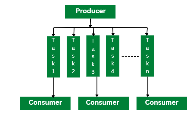
Parallel LU factorization algorithm

As shown in the above diagram, the Parallel LU factorization algorithm uses the pipeline model. In this model, the producer reads the input matrix and generated the tasks that are required for computing the LU factorization as an output. The producer divides this input matrix into a smaller size of multiple tasks and shares them into a shared task queue. The consumers then retrieve these blocks and perform the LU factorization on each independent block.

6. Hybrid Model

A hybrid model is the combination of more than one parallel model. This combination can be applied sequentially or hierarchically to the different phases of the parallel algorithm. The model that can be efficient for performing the task is selected as a model for that particular phase.

Example: A combination of master-slave, work pool, and data graph model. 

 A combination of master slave, work pool and data graph model

As shown in the above hybrid model where three different models are used at each phase master-slave model, the work pool model, and the data graph model. Consider the above example where the master-slave model is used for the data transformation task. The master process distributes the task to multiple slave processes for parallel computation. In the second phase work pool model is used for data analysis and similarly data graph model is used for making the data visualization. In this way, the operation is carried out in multiple phases and by using different parallel algorithm models at each phase.

Conclusion

The parallel algorithm model solves the large problem by dividing it into smaller parts and then solving each independent sub-task simultaneously by using its own approach. Each parallel algorithm model uses its own data partitioning and data processing strategy. However, the use of these parallel algorithm models improves the speed and efficiency of solving a particular task.