Orthogonal Matching Pursuit (OMP) using Sklearn

In this article, we will delve into the Orthogonal Matching Pursuit (OMP), exploring its features and advantages.

What is Orthogonal Matching Pursuit?

The Orthogonal Matching Pursuit (OMP) algorithm in Python efficiently reconstructs signals using a limited set of measurements. OMP intelligently selects elements from a “dictionary” to match the signal, operating in a stepwise manner. The process continues until a specified sparsity level is reached or the signal is adequately reconstructed. OMP’s versatility is evident in applications like compressive sensing, excelling in pinpointing sparse signal representations. Its implementation in Python, through sklearn.linear_model.OrthogonalMatchingPursuit, proves valuable in image processing and feature selection.

In this analogy, Python’s Orthogonal Matching Pursuit (OMP) is likened to a detective’s toolkit for reconstructing missing elements in a signal, resembling solving a puzzle with absent pieces. OMP identifies the most significant signal elements, starting with an empty guess and iteratively selecting the best-fitting pieces from measurements. This iterative process refines the approximation until the essential components of the signal are revealed. Implemented in Python using sklearn.linear_model.OrthogonalMatchingPursuit`, OMP acts as a detective guiding the uncovering of crucial elements and completing the signal puzzle.

Steps Needed

• Initialization:
  • Initialize the residual signal r as the original signal.
  • Initialize the support set T as an empty set.
• Iteration:
  • Find the index of the atom most correlated with the current residual.
  • Update the support set T by adding the index of the selected atom.
  • Solve a least-squares problem using the atoms from the current support set to update the coefficients.
  • Update the residual signal.
• Termination:
  • Repeat the iteration until a predefined number of iterations or until the residual becomes sufficiently small.

Orthogonal Matching Pursuit Using Scikit-learn

In this example below code uses scikit-learn to apply Orthogonal Matching Pursuit (OMP) for sparse signal recovery. It generates a random dictionary matrix and a sparse signal, then observes the signal. OMP is applied with a specified number of expected non-zero coefficients. The results include the estimated coefficients and the support set (indices of non-zero coefficients), providing information about the original and estimated sparse signals.

Python3

from sklearn.linear_model import OrthogonalMatchingPursuit
import numpy as np

# Step 1: Generate or Load Data
# Let's create a dictionary (matrix Phi) and a sparse signal (vector x)
# Dictionary matrix with 10 atoms of dimension 20
Phi = np.random.randn(10, 20)
x = np.zeros(20)
# Sparse signal with non-zero coefficients at indices 2, 5, and 8
x[[2, 5, 8]] = np.random.randn(3)
# Observed signal
y = np.dot(Phi, x)

# Step 2: Apply Orthogonal Matching Pursuit
# Specify the expected number of non-zero coefficients
omp = OrthogonalMatchingPursuit(n_nonzero_coefs=3)
omp.fit(Phi, y)

# Step 3: Get Results
coefficients = omp.coef_  # Estimated coefficients
# Indices of non-zero coefficients
support_set = np.where(coefficients != 0)[0]

# Display Results
print("Original Sparse Signal:\n", x)
print("\nEstimated Sparse Signal:\n", coefficients)
print("\nIndices of Non-Zero Coefficients (Support Set):", support_set)

Output:

Original Sparse Signal:
 [ 0.          0.         -0.60035931  0.          0.          0.06069191
  0.          0.         -0.65530325  0.          0.          0.
  0.          0.          0.          0.          0.          0.
  0.          0.        ]

Estimated Sparse Signal:
 [-0.14809913  0.          0.          0.          0.          0.
  0.          0.         -1.03167779  0.          0.         -0.16831767
  0.          0.          0.          0.          0.          0.
  0.          0.        ]

Indices of Non-Zero Coefficients (Support Set): [ 0  8 11]

Sparse Signal Recovery using Orthogonal Matching Pursuit

In this example below code illustrates sparse signal recovery using Orthogonal Matching Pursuit (OMP). It generates a sparse signal with non-zero coefficients, creates an observed signal by multiplying it with a random matrix (dictionary), and applies OMP for signal recovery. The recovered and true sparse signals are then plotted for visual comparison.

Python

from sklearn.linear_model import OrthogonalMatchingPursuit
import numpy as np
import matplotlib.pyplot as plt

# Set random seed for reproducibility
np.random.seed(42)

# Step 1: Generate a sparse signal
signal_length = 100
sparse_signal = np.zeros(signal_length)
sparse_signal[[10, 30, 50, 70]] = [3, -2, 4.5, 1.2]  # Non-zero coefficients

# Step 2: Generate a measurement matrix (dictionary)
measurement_matrix = np.random.randn(50, signal_length)

# Step 3: Create the observed signal with noise
noise_level = 0.5
observed_signal = np.dot(measurement_matrix, sparse_signal) + noise_level * np.random.randn(50)

# Step 4: Apply OMP for signal recovery
omp = OrthogonalMatchingPursuit(n_nonzero_coefs=4)
omp.fit(measurement_matrix, observed_signal)
recovered_signal = omp.coef_

# Step 5: Plot the results
plt.figure(figsize=(12, 3))

# Original Sparse Signal
plt.subplot(1, 3, 1)
plt.stem(sparse_signal, basefmt='r', label='Original Sparse Signal')
plt.title('Original Sparse Signal')
plt.legend()

# Observed Signal
plt.subplot(1, 3, 2)
plt.stem(observed_signal, basefmt='b', label='Observed Signal with Noise')
plt.title('Observed Signal with Noise')
plt.legend()

# Recovered Sparse Signal
plt.subplot(1, 3, 3)
plt.stem(recovered_signal, basefmt='g', label='Recovered Sparse Signal')
plt.title('Recovered Sparse Signal using OMP')
plt.legend()

plt.tight_layout()
plt.savefig('omp.png')
plt.show()

Output:

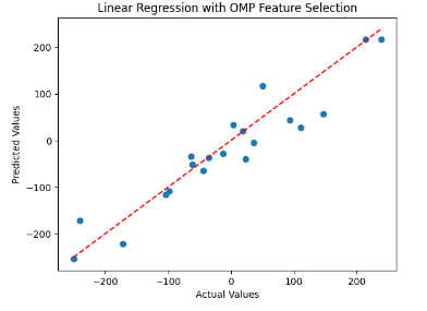
Orthogonal Matching Pursuit for Feature Selection in Linear Regression

In this example below code showcases a regression workflow with scikit-learn. It generates synthetic data, splits it, applies Orthogonal Matching Pursuit for feature selection, trains a linear regression model, and evaluates its performance on a test set. The script concludes with a scatter plot visualizing the accuracy of the regression model.

Python

from sklearn.linear_model import OrthogonalMatchingPursuit
from sklearn.datasets import make_regression
from sklearn.model_selection import train_test_split
from sklearn.linear_model import LinearRegression
import numpy as np
import matplotlib.pyplot as plt

# Generate synthetic data for regression
X, y = make_regression(n_samples=100, n_features=20, noise=5, random_state=42)

# Split the data into training and testing sets
X_train, X_test, y_train, y_test = train_test_split(X, y, test_size=0.2, random_state=42)

# Apply OMP for feature selection
omp = OrthogonalMatchingPursuit(n_nonzero_coefs=5)
omp.fit(X_train, y_train)

# Train a linear regression model using the selected features
selected_features = np.where(omp.coef_ != 0)[0]
X_train_selected = X_train[:, selected_features]
X_test_selected = X_test[:, selected_features]

lr = LinearRegression()
lr.fit(X_train_selected, y_train)

# Evaluate the model on the test set
y_pred = lr.predict(X_test_selected)

# Plot the predicted vs actual values
plt.scatter(y_test, y_pred)
plt.plot([min(y_test), max(y_test)], [min(y_test), max(y_test)], linestyle='--', color='red')
plt.xlabel('Actual Values')
plt.ylabel('Predicted Values')
plt.title('Linear Regression with OMP Feature Selection')
plt.show()

Output:

Linear Regression using OMP

Advantages of Orthogonal Matching Pursuit (OMP)

There are numerous advantages to OMP, and we will highlight some key examples.

• Sparsity Preservation: OMP excels in accurately recovering sparse signals, ensuring the preservation of the underlying signal’s sparsity. This feature proves particularly effective for applications characterized by a limited number of non-zero coefficients.
• Adaptive Model Complexity: OMP provides flexibility in selecting the number of non-zero coefficients. Users can specify the desired sparsity level, and OMP automatically adjusts the model complexity to align with the inherent sparsity of the signal.
• Iterative Refinement: Through an iterative process, OMP continuously refines sparse signal estimates by incrementally adding atoms to the support set. This iterative refinement enhances the precision of sparse signal recovery.
• Computational Efficiency: OMP stands out for its computational efficiency, especially when compared to certain optimization-based sparse recovery methods. By solving a series of least-squares problems, OMP proves to be less computationally demanding than more intricate optimization procedures.
• Flexibility in Dictionary Design: OMP’s versatility is evident in its ability to work with various dictionaries, including overcomplete dictionaries. This adaptability makes it a valuable tool for diverse signal processing application

Conclusion

In summary, Orthogonal Matching Pursuit (OMP) emerges as a powerful and efficient algorithm for sparse signal recovery. Its simplicity, coupled with the ability to select relevant atoms while maintaining orthogonality, makes it a popular choice in compressive sensing and image processing. Despite some challenges, OMP remains a valuable tool in signal processing, providing a computationally feasible approach for extracting meaningful information from sparse data representations.