networkD3 package in R

networkD3: Data-driven document Network, is an R package for creating network graphs which are used for 3-Dimensional visualizations of data as network graphs. In R Programming Language It was created using the HTML widget package in javascript by Christopher Gandrud et.al, Using (>=v0.99) this version of Rstudio the graph will appear on the viewer pane. Not only appear but also gives us a handy way of seeing and tweaking our network graphs. This package helps understand the network connections between nodes. Moreover, if you want to extract the graph from Rstudio you can export the graph to the clipboard or PNG/JPEG/etc.

Note: You are used to R’s 1-based indexing (i.e. counting in R starts from 1). However, networkD3 plots are created using JavaScript, which is 0-based indexing so, your data links will need to start from 0

In the ,networkD3 package there are many functions. Following are the popular network functions used by many.

• Simple Network
• Force Network
• Sankey Network
• Radial Network
• Dendro Network
• Chord Network

INSTALLATION:

To use a package in R programming we have to install the package first. For installing the R package in R studio use the command install.packages(“name”). Follow the following steps to get the packages installed on your system.

install.packages('networkD3')

SIMPLE NETWORK

A simple network is a basic form of a Forced-directed network, we can use Force network to create a Simple network by providing appropriate data and customization options. For a simple form of a Force-directed network, we can use a simple network (). It works based on a “node-link” diagram and is connected by edges. It provides us with amazing animation with an intuitive way of observing data and also allows us to tweak the networks with cursors. The purpose of the simple network is to provide a good understanding of difficultly visualized data. It is used to represent simple connections like social media connections, biological connections(Genes, Proteins,..), etc, It contains few network connections compared to the force network since it’s the base variant of the force-directed network.

SYNTEX

simpleNetwork(Data, Source = 1, Target = 2, height = NULL, width = NULL, linkDistance = 50
,charge = -30, fontSize = 7, fontFamily = "serif",   linkColour = "#666", 
nodeColour = "#3182bd",opacity = 0.6, zoom = F)

ARGUMENTS:

• Data – A data frame with three columns. The first two are the names of the linked node. The third column is an edge value.
• Source – If Source = NULL then the first column of the data frame is treated as the source. Network source variable in the data frame.
• Target – If Target = NULL, then the data frame’s second column is treated as the target. Network target variable in the data frame.
• height – Height for the network graph’s frame area in pixels.
• width – Width for the network graph’s frame area in pixels.
• link distance – The Numeric distance between the links in pixels.
• charge – The Numeric value indicates either the node repulsion’s strength (negative value) or attraction (positive value).
• font Size – The Numeric font size in pixels for the node text labels.
• font Family – Font family for the node text labels.
• linkColour – A Character string defining the color you want the link lines to be.
• nodeColour – A Character string defining the color you want the node circles to be.
• opacity – The Numeric value of the proportion opaque you would like the graph elements to be.
• zoom – Logical value ( ‘TRUE’ – enable, ‘FALSE’ – disable ).

Example
For Instance, we have a group of five friends named Sam, Sai, Robert, Tom, and Murphy. They are talking and sharing some information among themselves this simple conversation among those friends is represented as edges and the five friends are represented as nodes. This scenario of discussion among them can be visualized in a simple network.

R

# Load package
library(networkD3)

# Create data
X <- c("A","A","A","A",
       "B","C","B","D","C")
Y <- c("C","B","D","E",
       "K","J","G","H","I")
networkData <- data.frame(X,Y)

# Plot
simpleNetwork(networkData, fontFamily='fantasy', nodeColour = 'green')

Output:

NetworkD3

• Install the package and load the package “networkD3” using the library(networkD3).
• Create a variable X and store a set of data as a vector.
• Create another variable Y and store a set of other data as a vector.
• Create a dataframe using data. frame(X, Y) to store X and Y values and store them in the networkData variable.
• Use simple network () to plot the data as a network graph, network data is the input data, ‘fantasy’ is the font family, and ‘green’ is the node color.

FORCE NETWORK

A Force network is also known as node-link diagram though it is useful for visualizing networks with nodes and edges which are connected by forces. Force network provides wonderful animations for understanding the network’s data element and also allows us to tweak the data in a repulsive and attractive manner. For the complex form of a forced-directed network and to have more control over the appearance of the forced-directed network we can use force network (). It contains more network connections than a simple network since it’s the extension variant of the forced-directed network.

SYNTAX:

forceNetwork(Links, Nodes, Source, Target, Value, NodeID, Nodesize, Group,height = NULL,
width = NULL,   colourScale = JS("d3.scaleOrdinal(d3.schemeCategory20);"), fontSize = 7,
fontFamily = "serif", linkDistance = 50,   linkWidth = JS("function(d) 
{ return Math.sqrt(d.value); }"),
radiusCalculation = JS(" Math.sqrt(d.nodesize)+6"), 
charge = -30,linkColour = "#666", opacity = 0.6, zoom = FALSE, legend = FALSE,
arrows = FALSE, bounded = FALSE, opacityNoHover = 0,clickAction = NULL)

ARGUMENTS:

• Links – A data frame object with the links between the nodes. It should include the Source and Target for each link. An optional Value variable can be included to specify how close the nodes are to one another.
• Nodes – A data frame containing the node id and properties of the nodes. If no ID is specified then the nodes must be in the same order as the Source variable column in the Links data frame.
• Source – Character string naming the network source variable in the Links data frame.
• Target – Character string naming the network target variable in the Links data frame.
• Value – Character string naming the variable in the Links data frame for the links’ width.
• NodeID – Character string specifying the node IDs in the Nodes data frame.
• Nodesize – Character string specifying the column in the Nodes data frame with some value to vary the node radii with. See also radiusCalculation.
• Group – Character string defining the group of each node in the Nodes data frame.
• height – Numeric height for the network graph’s frame area in pixels.
• width – Numeric width for the network graph’s frame area in pixels.
• colourScale – Character string defining the categorical color scale for the nodes.
• font Size – Numeric font size in pixels for the node text labels.
• font Family – Font family for the node text labels. e indicating either the strength of the node repulsion (negative value) or attraction (positive value).
• linkColour – Character vector specifying the color you want the link lines to be.
• opacity – The numeric value of the proportion opaque you would like the graph elements to be.
• zoom – Logical value ( ‘TRUE’ – enable, ‘FALSE’ – disable ).
• legend – Logical value ( ‘TRUE’ – enable, ‘FALSE’ – disable ).
• arrows – Logical value ( ‘TRUE’ – enable, ‘FALSE’ – disable ).
• bounded – Logical value ( ‘TRUE’ – enable, ‘FALSE’ – disable ).
• opacityNoHover – Numeric value of the opacity proportion for node labels text when the mouse is not hovering over them.
• clickAction – A character string with a JavaScript expression to evaluate when a node is clicked.

EXAMPLE

For instance consider there is a lakh of people living in a city with their friends, and families. The activity of contacting, sharing, and connecting among them can be represented as edges and the people, their friends, and their families are represented as nodes. The scenario of connection among a lack of people can be visualized using a force network.

R

# Load data
data(MisLinks)
data(MisNodes)

# Plot
forceNetwork(Links = MisLinks, Nodes = MisNodes,
             Source = "source", Target = "target",
             Value = "value", NodeID = "name",
             Group = "group", opacity = 1)
forceNetwork()

Output:

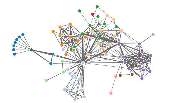
NetworkD3

The ‘MisLinks’ and ‘MisNodes’ are an example of datasets in the ‘networkD3’ package that provides a simulated network of links (edges). MisLinks dataset contains columns such as ‘source’, ‘target’, and ‘value’ that describes the source nodes, target nodes, and the strength of the links. MisNodes dataset contains columns such as ‘name’, ‘group’, and ‘size’ that describes the node names, grouping, and sizes.

• Load the ‘MisLinks’ dataset using data(MisLinks).
• Load the ‘MisNodes’ dataset using data(MisNodes).
• Create a force network using forceNetwork(), assign MisLinks for Links, MisNodes for Nodes, ‘source’ column for Source, ‘target’ column for Target, ‘value’ column for Value, ‘name’ column for NodeID, ‘group’ column for Group and assign value ‘1’ for opacity.
• Call the network using forceNetwork().

SANKEY NETWORK

A Sankey network is a type of visualization that shows the flows and movement of objects between nodes of different categories or groups. Sankey is useful for understanding the transition, distribution, or transformation of quantities or values within a system. It also consists of nodes and links. It is a complex form of network in the networkD3 package because of the massive network components. The link in the Sankey network is of different sizes according to the data flow through the link. The width of the links represents the magnitude or volume of the flow.

SYNTAX:

sankeyNetwork(Links, Nodes, Source, Target, Value, NodeID, NodeGroup = NodeID,
LinkGroup = NULL, units = "",   colourScale = JS("d3.scaleOrdinal(d3.schemeCategory20);"),
fontSize = 7,   fontFamily = NULL, nodeWidth = 15, nodePadding = 10, margin = NULL, 
height = NULL, width = NULL, iterations = 32, sinksRight = TRUE)

ARGUMENTS:

• Links – A data frame object with the links between the nodes. It should include the Source and Target for each link. An optional Value variable can be included to specify how close the nodes are to one another.
• Nodes – A data frame containing the node id and properties of the nodes. If no ID is specified then the nodes must be in the same order as the Source variable column in the Links data frame.
• Source – A character string naming the network source variable in the Links data frame.
• Target – A character string naming the network target variable in the Links data frame.
• Value – A character string naming the variable in the Links data frame for how wide the links are.
• NodeID – A character string specifying the node IDs in the Nodes data frame.
• NodeGroup – A character string specifying the node groups in the Nodes.
• LinkGroup – A character string specifying the groups in the Links. Used to color the links in the network.
• units – A character string describing physical units for Value.
• color Scale – A character string specifying the categorical color scale for the nodes.
• font Size – The numeric font size in pixels for the node text labels.
• font Family – Font family for the node text labels.
• nodeWidth – The numeric width of each node.
• nodePadding – The numeric essentially influences the width height.
• margin – An integer or a named list/vector of integers for the plot margins.
• height – The numeric height for the network graph’s frame area in pixels.
• width – The numeric width for the network graph’s frame area in pixels.
• iterations – Numeric. Number of iterations in the diagram layout for computation of the depth (y-position) of each node
• sinks Right – Logical(TRUE- last nodes are moved to the right border of the plot).

EXAMPLE:

Consider there is a number of industries, transportation, aviation, living areas, etc., that need resources like gas, oil, electricity, etc., for their existence and surveillance. Then the industries, transportation, gas, oil, etc., are represented as nodes of the network, and the connections among them can be represented as links(edges) of the network, If we require the amount of usage of the resources used by industries then we can use Sankey network.

R

library(networkD3)

# Load energy projection data
URL <- paste0('https://cdn.rawgit.com/christophergandrud/networkD3/',
              'master/JSONdata/energy.json')
energy <- jsonlite::fromJSON(URL)

# Colour Nodes
sankeyNetwork(Links = energy$links, Nodes = energy$nodes, Source = 'source',
              Target = 'target', Value = 'value', NodeID = 'name',
              units = 'TWh', fontSize = 12, nodeWidth = 30)

# Colour links
energy$links$energy_type <- sub(' .*', '',
                                energy$nodes[energy$links$source + 1, 'name'])

sankeyNetwork(Links = energy$links, Nodes = energy$nodes, Source = 'source',
              Target = 'target', Value = 'value', NodeID = 'name',
              LinkGroup = 'energy_type', NodeGroup = NULL)

Output:

NetworkD3

“jsonlite::fromJSON” is a function in “jsonlite” package in R that is used to convert JSON data in R objects that represents the JSON data. In the above program, jsonlite::fromJSON(URL) is a function in ‘jsonlite’ package that converts the JSON formatted data into R objects and stores it in the ‘energy’ variable.

• Load the library “networkD3” using load(“library”).
• Create a variable ‘URL’ and concatenate both the URLs.
• Create a variable ‘energy’ and store a json formatted data.
• Create a Sankey network using sankeyNetwork() and assign links, nodes, sources, targets, values, and NodeID.
• Again create a Sankey network but this time adds LinkGroup = ‘energy_type’ to get a colorful link in the network.

RADIAL NETWORK:

A radial network also known as the is Reingold-Tilford Tree network, is a type of network visualization where nodes are arranged in a circular or radial layout. In a , radial network the root node is the center present at the centre of the network and the parent node present at is outside of the circular graph. Radial network visualization is particularly useful when we want to display hierarchical relationships between nodes, such as organizational structures, family trees, or classification hierarchies.

SYNTAX:

radialNetwork(List, height = NULL, width = NULL, fontSize = 10, fontFamily = "serif",
linkColour = "#ccc", nodeColour = "#fff",  nodeStroke = "steelblue", textColour = "#111", 
opacity = 0.9, margin = NULL)

ARGUMENTS:

• List – A hierarchical list object with a root node and children.
• height – Numeric height for the network graph’s frame area in pixels.
• width – Numeric width for the network graph’s frame area in pixels.
• font Size – Numeric font size in pixels for the node text labels.
• font Family – Font family for the node text labels.
• link Colour – A character string specifying the color you want the link lines to be.
• node Colour – A character string specifying the color you want the node circles to be.
• nodeStroke – A character string specifying the color you want the node perimeter to be.
• textColour – A character string specifying the color you want the text to be before they are clicked.
• opacity – The numeric value of the proportion opaque you would like the graph elements to be.
• margin – An integer or a named list/vector of integers for the plot margins.

EXAMPLE:
For example, consider there is a group of employees working in an organization for the development of the firm. So, they require communication in a circulated manner for sharing of information among them. For this type of scenario, we can use a Radial network(tree network). An organization manager, employer, employee, HR, etc., can be represented as a node of the network and the sharing of information among them and their relationship can be represented as the links(edges).

R

#Load library
library(networkD3)
Data <- paste0(
        "https://cdn.rawgit.com/christophergandrud/networkD3/",
        "master/JSONdata//flare.json")

## Convert to a list format
Flare <- jsonlite::fromJSON(Data, simplifyDataFrame = FALSE)

# Use a subset of data for more readable diagram
Flare$children = Flare$children[1:3]

radialNetwork(List = Flare, fontSize = 10, opacity = 0.9)
radialNetwork

Output:

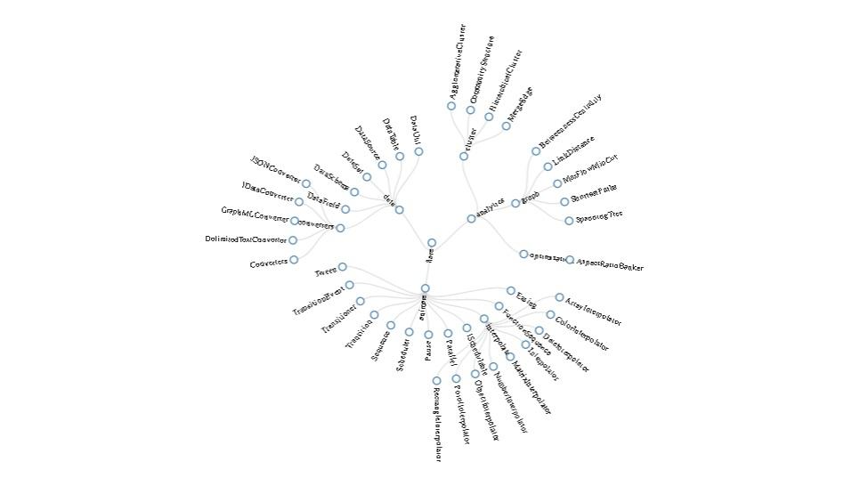
RADIAL NETWORK

• Load the library using library(networkD3).
• Create a variable ‘Data’ and concatenate both the URLs.
• Create a variable ‘Flare’ and store a json formated data.
• Create a radial network using radialNetwork() and assign the values “Flare” to List, add fontSize 10, add opacity 0.9.

DENDRO NETWORK

The Dendro network is a network visualization that uses a hierarchical type of visualization of data. It is particularly useful when visualizing `hierarchical clustering or tree structures. It contains the root node where the tree graph starts and the parent node where the tree graph ends. It can help for understanding complex information through network visualization.

SYNTAX:

dendroNetwork(hc, height=500, width=800, fontSize=10, linkColour="#ccc",nodeColour="#fff",
nodeStroke="steelblue",  textColour="#111", textOpacity=0.9,textRotate=NULL, opacity=0.9,
margins=NULL, linkType=c("elbow", "diagonal"),
treeOrientation=c("horizontal", "vertical"), zoom=FALSE)

ARGUMENTS:

• hc – A hierarchical (hclust) cluster object.
• height – The numeric height for the network graph’s frame area in pixels.
• width – The numeric width for the network graph’s frame area in pixels.
• fontSize – The numeric font size in pixels for the node text labels.
• linkColour – A character string specifying the colour you want the link lines to be.
• nodeColour – A character string specifying the colour you want the node circles to be.
• nodeStroke – A character string specifying the color you want the node perimeter to be.
• textColour – A character string specifying the color you want the text to be before they are clicked.
• textOpacity – The numeric vector or scalar of the proportion opaque you would like the text to be before they are clicked.
• textRotate – The numeric degrees to rotate text for node text. The default is 0 for horizontal and 65 degrees for vertical.
• opacity – The numeric value of the proportion opaque you would like the graph elements to be.
• margins – An integer or a named list/vector of integers for the plot margins.
• linkType – Character specifying the link type between points.
• treeOrientation – Character specifying the tree orientation(“vertical”,”horizontal”).
• zoom – Logical value ( ‘TRUE’ – enable, ‘FALSE’ – disable ).

EXAMPLE:
Consider there is a family consisting of family members and their ancestors, If a Researcher want to collect ancient data about a family like their ancestors related details and he/she wants to visualize those data in an understandable and structured form. In this type of scenario, a Researcher can choose Dendro Network. The family members, their parents, their grandparents, their great grandparents, etc., can be represented as nodes of the network, and the relationship links between them can be represented as edges.

R

#Load library
library(networkD3)

#Creating data
hc <- hclust(dist(USArrests), method="ave")

#dendro_network
dendroNetwork(hc,textColour=c("red","green","orange")[cutree(hc,3)], height=600)

Output:

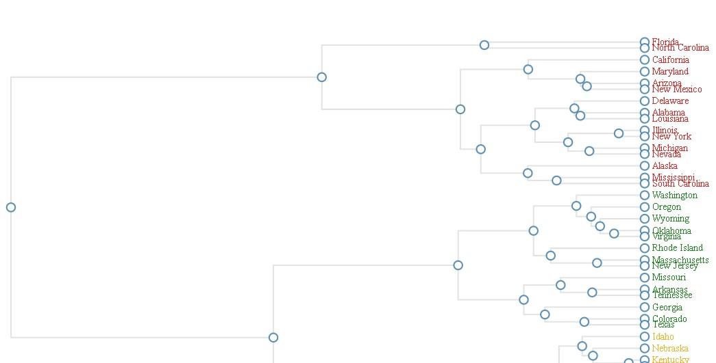
DENDRO NETWORK

• Load the library using library(networkD3).
• Creating US crime data as in hierarchical cluster format.
• Create dendro network using dendroNetwork(), assign hierarchical cluster variable to hc, add textColour, cut down the tree using cutree() and assign 600 to height.

CHORD NETWORK

A Chord network is also known as a circular network. It is a type of network visualization that represents relationships and connections between entities or categories. It is particularly useful for showing the interactions and associations between different groups or entities. In a chord network, entities or groups are represented as arcs on a circle, and the connections or relationships are displayed as chords connecting the arcs. The width of the chords can be used to represent the strength, magnitude, or frequency of the connections.

SYNTAX:

chordNetwork(Data, height=500, width=500, initialOpacity=0.8, useTicks=0,colourScale=NULL,
padding=0.1, fontSize=14, fontFamily="sans-serif", labels=c(), labelDistance=30)

ARGUMENTS:

• Data – A square matrix or dataframe whose (n,m) entry represents the strength of the link from group n to group m.
• height – Height for the network graph’s frame area in pixels.
• width – Numeric width for the network graph’s frame area in pixels.
• initialOpacity – Specify the opacity before the user mouses over the link.
• useTicks – Integer number of ticks on the radial axis.
• colourScale – Specify the hexa decimal colors in which to display the different categories.
• padding – Specify the amount of space between adjacent categories on the outside of the graph.
• font Size – Numeric font size in pixels for the node text labels.
• font Family – Font family for the node text labels.
• labels – Vector containing labels of the categories.
• label distance – Integer distance in pixels(px) between text labels and outer radius. ’30’ is the default value.

EXAMPLE:
In supply chain marketing, Chord diagrams can be used to visualize supply chain relationships, showing connections between suppliers, manufacturers, distributors, and customers. This can help identify dependencies, bottlenecks, and potential improvements in the supply chain.

R

#Load the library
library(networkD3)

#Create data
hairColourData<-matrix(c(11975,1951,8010,1013,
                         5871,10048,16145,990,
                         8916,2060,8090,940,
                         2868,6171,8045,6907),
                         nrow=4)

#Create chord diagram
chordNetwork(Data=hairColourData,
             width=500,
             height=500,
             colourScale=c("#000000", "#FFDD89", "#957244", "#F26223"),
             labels=c("red","brown","blond","gray"))

Output:

chord Network

• Load the library using library(networkD3).
• Create matrix of data about hair colour and store it in ‘hairColourData’ variable.
• Create chord network using chordNetwork() with ‘hairColourData’ as Data, 500 as width and height, finally add colours and labels of colours.

SAVING NETWORK GRAPH AS HTML FILE

If you want to save your network in an HTML file you can use saveNetwork it after the network implementation. The function saveNetwork is from the library ‘magrittr’. Using the below R code in Rstudio we can save the network of any type in our system as HTML, JPEG, or PNG file

R

library(magrittr)

simpleNetwork(networkData) %>%
saveNetwork(file = 'Net1.html')