Multiple Linear Regression using R to predict housing prices

Predicting housing prices is a common task in the field of data science and statistics. Multiple Linear Regression is a valuable tool for this purpose as it allows you to model the relationship between multiple independent variables and a dependent variable, such as housing prices. In this article, we’ll walk you through the process of performing Multiple Linear Regression using R Programming Language to predict housing prices.

Multiple Linear Regression

Multiple Linear Regression is an extension of simple linear regression, which models the relationship between a single independent variable and a dependent variable. In the case of predicting housing prices, we typically have “several independent variables”, like the number of bedrooms, square footage, location, and so on. Multiple Linear Regression allows us to incorporate all these factors into our model.

In the context of Multiple Linear Regression, the equation to predict housing prices can be expressed as.

Where:

• Y is the dependent variable (housing price).
• is the intercept.
• are the coefficients of the independent variables.
• are the independent features
• represents the error term

Data Preparation

Before diving into Multiple Linear Regression, you need a dataset that contains information on housing prices and relevant independent variables.

R provides many ways to import data, but for the purposes of this article, we will assume you have a CSV file (housing_data.csv) containing the necessary data or you can download it from here.

Load the data

You can load your dataset into R using the read.csv() function, and check its dimensions (rows and columns) using dim() function.

R

data <- read.csv("housing_data.csv")
dim(data)

Ouptut

[1] 2919   13

Displaying the initial 10 data rows using the View() function.

R

head(data)

Output:

  MSSubClass MSZoning LotArea LotConfig BldgType OverallCond YearBuilt
1         60        4    8450         5        1           5      2003
2         20        4    9600         3        1           8      1976
3         60        4   11250         5        1           5      2001
4         70        4    9550         1        1           5      1915
5         60        4   14260         3        1           5      2000
6         50        4   14115         5        1           5      1993
  YearRemodAdd Exterior1st BsmtFinSF2 TotalBsmtSF SalePrice
1         2003          13          0         856    208500
2         1976           9          0        1262    181500
3         2002          13          0         920    223500
4         1970          14          0         756    140000
5         2000          13          0        1145    250000
6         1995          13          0         796    143000

Data Cleaning

Observing the preceding visualization, it’s evident that the dataset includes <NA> or Null values, necessitating data cleaning.

To identify “Which columns have null values and how many?” I intend to craft a function called getMissingValues(). This function will compute and display the columns and their corresponding count of missing values, sorted in descending order from the most to the least.

R

getMissingValues <- function(data) {
  # Check for missing values in each column and store the result
  missing_values <- colSums(is.na(data))

  # Sort the columns by the number of missing values in descending order
  sorted_missing_values <- sort(missing_values, decreasing = TRUE)

  # Display the sorted missing values and their corresponding column names
  for (col_name in names(sorted_missing_values)) {
    cat("Column:", col_name, "\tMissing Values:", sorted_missing_values[col_name], "\n")
  }
}

getMissingValues(data)

Output

Column: SalePrice     Missing Values: 1459 
Column: BsmtFinSF2     Missing Values: 1 
Column: TotalBsmtSF     Missing Values: 1 
Column: Id     Missing Values: 0 
Column: MSSubClass     Missing Values: 0 
Column: MSZoning     Missing Values: 0 
Column: LotArea     Missing Values: 0 
Column: LotConfig     Missing Values: 0 
Column: BldgType     Missing Values: 0 
Column: OverallCond     Missing Values: 0 
Column: YearBuilt     Missing Values: 0 
Column: YearRemodAdd     Missing Values: 0 
Column: Exterior1st     Missing Values: 0

Columns SalePrice, BsmtFinSF2 and TotalBsmtSF have missing values.

Filling missing values

The initial action taken is the filling of rows containing missing values. we will fill the missing values with mean.

R

# Remove missing values
data<-na.omit(data)
sum(is.na(data))

Output:

[1] 0

Dropping ID column

subset(data, select = -Id) is the function call. It instructs R to create a subset of the dataset, excluding the “Id” column.

The select argument, set to -Id, specifies that we want to retain all columns except for the one named “Id.” In R, when you use a minus sign in front of a column name within select, it effectively means “exclude this column.”

R

# Dropping id coulmn
data <- subset(data, select = -Id)

Label Encoding

I performed label encoding on categorical columns “MSZoning,” “LotConfig,” “BldgType,” and “Exterior1st” to convert their values into numeric representations.

This encoding is beneficial for machine learning algorithms, as they often require numeric inputs, making it easier to work with categorical data. By converting these categorical variables into numeric factors, I ensured that the model can use this information effectively in the predictive process.

R

# Performing label encoding
data$MSZoning <- as.numeric(factor(data$MSZoning))
data$LotConfig <- as.numeric(factor(data$LotConfig))
data$BldgType <- as.numeric(factor(data$BldgType))
data$Exterior1st <- as.numeric(factor(data$Exterior1st))

Exploratory data analysis

Now we perform some Exploratory data analysis for this data set.

R

library(ggplot2)
library(ggcorrplot)

# Using ggcorrplot to get correlation between features
ggcorrplot(cor(data),hc.order = TRUE, lab = TRUE)

Output

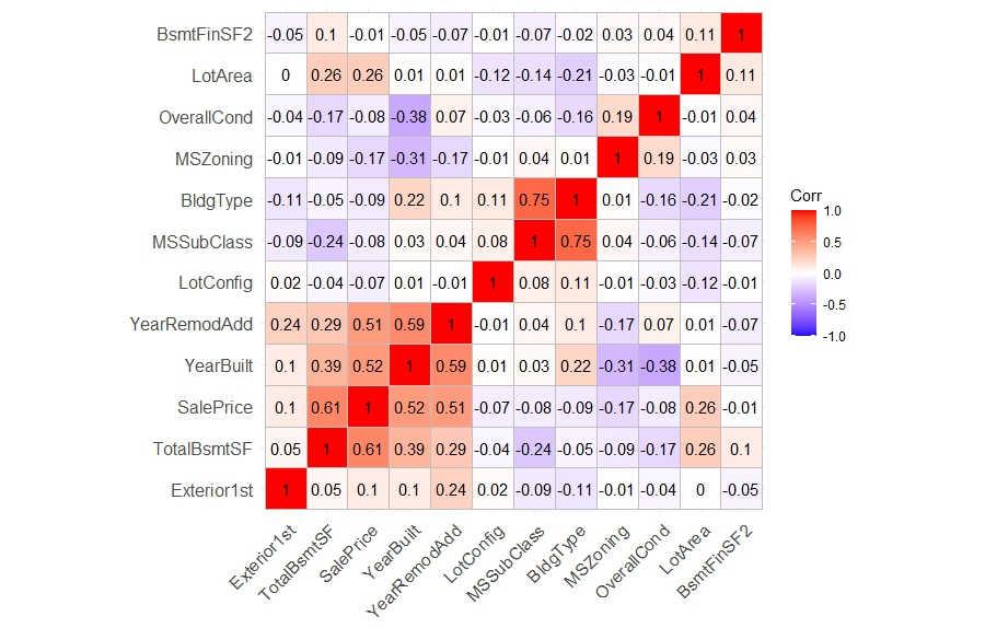
First, I installed the ggplot2 and ggcorrplot packages using the following commands.

• Once the packages were installed, I loaded them into my R session using the following commands:
• Next, I created a correlation matrix of my numeric data using the cor() function.
• Finally, I used the ggcorrplot() function to visualize the correlation matrix. I also specified the
• hc.order = TRUE argument to order the correlation matrix using hierarchical clustering
• lab = TRUE argument to display the variable labels on the plot.

The ggcorrplot() function produced a beautiful and informative correlation matrix plot. The plot showed the correlation coefficients between all pairs of variables in my data set, as well as the significance levels of the correlations. The plot also showed the hierarchical clustering of the variables, which helps us to identify groups of variables that were highly correlated with each other.

Sale price distribution

R

library(ggplot2)

# Create a histogram for a numeric variable (e.g., "Sale price") with aesthetic colors
ggplot(data, aes(x = SalePrice)) +
  geom_histogram(binwidth = 10000, fill = "skyblue", color = "darkblue") +
  labs(title = "Distribution of Price", x = "Price") +
  theme_minimal()

Output:

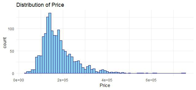
Distribution of Sale Price

First, I installed the ggplot2 package using the following command.

• Once the package was installed, I loaded it into my R session using the following command.
• Next, I created a histogram for the variable SalePrice with aesthetic colors using the following code.

The ggplot() function creates a new plot object.

• The aes() function maps aesthetic mappings to variables in the data set.
• The geom_histogram() function creates a histogram of the data.
• The binwidth argument specifies the width of the bins in the histogram.
• The fill argument specifies the fill color of the histogram bars. T
• he color argument specifies the line color of the histogram bars.
• The labs() function adds a title and x-axis label to the plot.
• The theme_minimal() function applies a minimalist theme to the plot.

Variation of Sale price with Lot area (Outlier detection)

R

# Create a scatter plot between "square_feet" and "price" with aesthetic colors
ggplot(data, aes(x = LotArea, y = SalePrice)) +
  geom_point(color = "red") +
  labs(title = "Scatter Plot: Lot area vs. Sale Price", x = "Lot area", y = "Sale Price") +
  theme_minimal()+
  geom_smooth(method = lm)

Output:

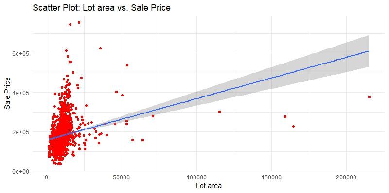
Scatter plot before removing outliers

The resulting plot is a scatter plot of the LotArea and SalePrice variables, with the points colored in red.

• The geom_smooth() function adds a fitted line to the scatter plot.
• The method argument specifies the method used to fit the line. In this case, I used the linear regression method (lm).

Scatter plot between “square_feet” and “price”

R

# Removing rows with Lot Area < 40000
data <- data[data$LotArea < 40000, ]

# Create a scatter plot between "square_feet" and "price" with aesthetic colors
ggplot(data, aes(x = LotArea, y = SalePrice)) +
  geom_point(color = "red") +
  labs(title = "Scatter Plot: Lot area vs. Sale Price", x = "Lot area", y = "Sale Price") +
  theme_minimal()+
  geom_smooth(method = lm)

Output

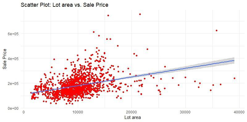
Scatter plot after removing outliers

The scatter plot shows that there are outliers in the data, which are skewing the regression line. To remove the outliers, we will remove all rows where the lot area is greater than 40,000 square feet.

We can then use this new dataset to fit a new regression line, which will be more representative of the overall trend in the data.

Building the Multiple Linear Regression Model

Since the data is now clean, we can generate a multiple linear regression model for it. To do this, we will split the data into two parts: a training set (70%) and a test set (30%).

Splitting data into train and test

R

# Splitting data into train and test
set.seed(123)

# Define the proportion for the training set (e.g., 70% for training, 30% for testing)
train_proportion <- 0.7

# Generate a random sample of row indices for the training set
train_indices <- sample(1:nrow(data),
                        size = round(train_proportion * nrow(data)))

# Create the training and testing datasets
train_data <- data[train_indices, ]
test_data <- data[-train_indices, ]

dim(train_data)

dim(test_data)

Output:

[1] 1012   12
[1] 434  12

Train multiple linear regression model

R

# Train a Multiple Linear Regression model on the train data
model <- lm(SalePrice ~ ., data = train_data)

# Printing summary of the model
summary(model)

Output

Call:
lm(formula = SalePrice ~ ., data = train_data)
Residuals:
    Min      1Q  Median      3Q     Max 
-162510  -25463   -5586   20765  271443 
Coefficients:
               Estimate Std. Error t value Pr(>|t|)    
(Intercept)  -3.046e+06  1.560e+05 -19.530  < 2e-16 ***
MSSubClass    5.702e+02  5.598e+01  10.184  < 2e-16 ***
MSZoning     -1.397e+03  2.324e+03  -0.601  0.54784    
LotArea       4.069e+00  3.874e-01  10.503  < 2e-16 ***
LotConfig     4.816e+02  9.052e+02   0.532  0.59481    
BldgType     -1.804e+04  2.088e+03  -8.642  < 2e-16 ***
OverallCond   5.904e+03  1.499e+03   3.937 8.81e-05 ***
YearBuilt     7.671e+02  7.372e+01  10.405  < 2e-16 ***
YearRemodAdd  7.833e+02  9.854e+01   7.950 5.03e-15 ***
Exterior1st  -8.116e+02  4.667e+02  -1.739  0.08235 .  
BsmtFinSF2   -2.334e+01  8.662e+00  -2.695  0.00716 ** 
TotalBsmtSF   8.961e+01  4.254e+00  21.067  < 2e-16 ***
---
Signif. codes:  0 ‘***’ 0.001 ‘**’ 0.01 ‘*’ 0.05 ‘.’ 0.1 ‘ ’ 1
Residual standard error: 45270 on 1000 degrees of freedom
Multiple R-squared:  0.6673,    Adjusted R-squared:  0.6637 
F-statistic: 182.4 on 11 and 1000 DF,  p-value: < 2.2e-16

• lm(formula = SalePrice ~ ., data = train_data) is the formula you used to fit the linear regression model. It indicates that you are regressing SalePrice on all available variables in the train_data dataset. The . represents “all variables except the dependent variable (SalePrice in this case).”
• Residuals: This section provides statistics about the residuals (the differences between the actual and predicted values) of the model. It includes the
• Coefficients:This section provides information about the estimated coefficients of the model for each independent variable. The coefficients represent the estimated effect of each variable on the dependent variable (SalePrice).
• Estimate represents the estimated coefficient value.
• Std. Error is the standard error of the coefficient estimate, which measures the uncertainty or variability of the estimate.
• t value is the t-statistic, which assesses the significance of the coefficient.
• Pr(>|t|) is the p-value associated with the t-statistic, indicating whether the coefficient is statistically significant.
• This represents the standard deviation of the residuals. It’s an estimate of the variability of the errors in the model.
• Multiple R-squared and Adjusted R-squared: The multiple R-squared is a measure of how well the independent variables explain the variance in the dependent variable (SalePrice).
• The adjusted R-squared takes into account the number of independent variables in the model and is often a more appropriate measure for comparing models with different numbers of variables. In this case, the adjusted R-squared is 0.6867, which means that the model explains approximately 68.67% of the variance in SalePrice.
• F-statistic:The F-statistic tests the overall significance of the model. It assesses whether at least one independent variable is significant in explaining the dependent variable. A small p-value (typically < 0.05) indicates that the model is significant ours p-value is less than 2.2e-16, thus the model has a good fit on the training data.

Model Prediction

R

predictions <- predict(model, newdata = test_data)

head(predictions)

Output

       1        3        7       14       15       21 
202136.0 216946.7 262690.4 250896.8 159607.4 254614.1 

We can use the predict() function to predict the sale price of the homes in the test set using the model that I trained on the train set. The predict() function takes two arguments: the model that I trained and the new data that I want to make predictions for. In this case, the new data is the test_data.

Predicting on a sample test

R

# Sample test case
test_case <- data.frame(MSSubClass = 60,MSZoning = 4,LotArea = 8450,
                        LotConfig = 5, BldgType = 1, OverallCond = 5,
                        YearBuilt = 2003, YearRemodAdd = 2003,
                        Exterior1st = 13, BsmtFinSF2 = 0,
                         TotalBsmtSF = 856
)

# Make predictions using the trained model
predicted_price <- predict(model, newdata = test_case)

# View the predicted price
print(predicted_price)

Output

     1 
202136

Visualizing predictions

To visualize prediction of our model, I’m using a function avPlots() (Added variable plots) which is a part of library ‘car’, to install it run install.packages(‘car’).

The avPlots() function produced a series of plots, one for each independent variable in the model. Each plot shows the relationship between the independent variable and the dependent variable, as well as the fitted regression line.

R

library(car)
avPlots(model)

Outputs

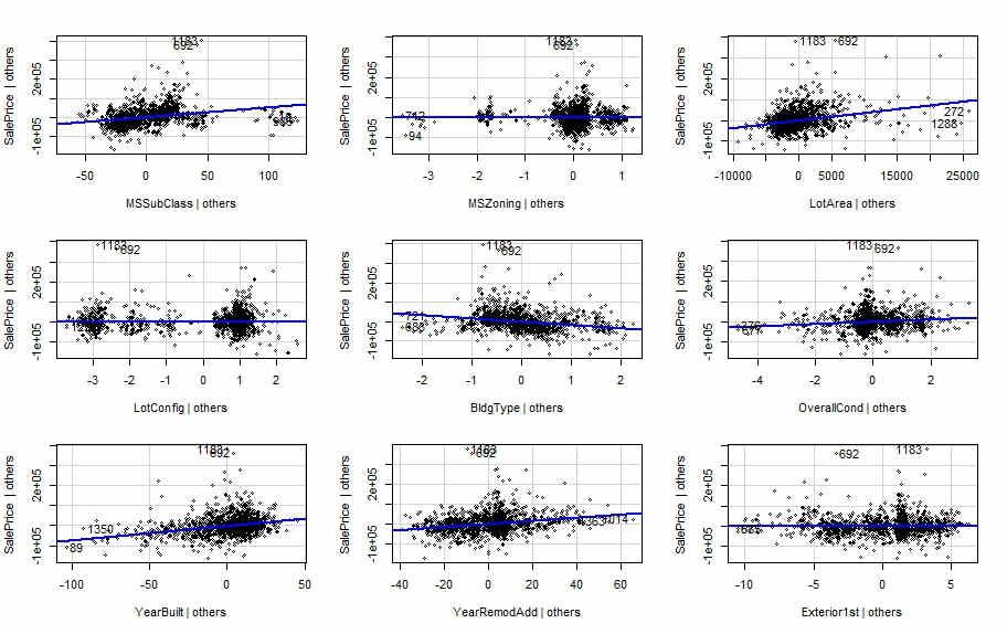
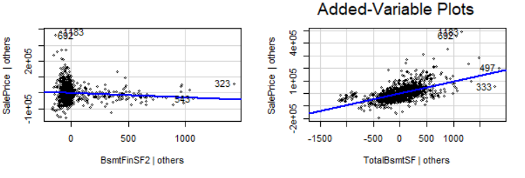
Overall,the results of the added-variable plots are satisfactory. They suggest that the multiple linear regression model is a good fit for the data, and that the model can be used to make accurate predictions about the sale price of new homes.

Conclusion

Multiple Linear Regression in R is a powerful tool for predicting housing prices by considering multiple factors simultaneously. It allows you to build a model that takes into account the impact of various independent variables on the dependent variable, providing a more accurate prediction of housing prices. However, remember that data quality, feature selection, and model evaluation are crucial aspects of the process. Careful attention to these steps will lead to a more reliable housing price prediction model.