ML | Multiple Linear Regression (Backward Elimination Technique)

Multiple Linear Regression is a type of regression where the model depends on several independent variables(instead of only on one independent variable as seen in the case of Simple Linear Regression). Multiple Linear Regression has several techniques to build an effective model namely:

• All-in
• Backward Elimination
• Forward Selection
• Bidirectional Elimination

In this article, we will implement multiple linear regression using the backward elimination technique.
Backward Elimination consists of the following steps:

• Select a significance level to stay in the model (eg. SL = 0.05)
• Fit the model with all possible predictors
• Consider the predictor with the highest P-value. If P>SL, go to point d.
• Remove the predictor
• Fit the model without this variable and repeat the step c until the condition becomes false.

Let us suppose that we have a dataset containing a set of expenditure information for different companies. We would like to know the profit made by each company to determine which company can give the best results if collaborated with them. We build the regression model using a step by step approach.

Step 1 : Basic preprocessing and encoding

# import the necessary libraries
import pandas as pd
import numpy as np
from sklearn.model_selection import train_test_split

# import the dataset
df = pd.read_csv('50_Startups.csv')

# first five entries of the dataset
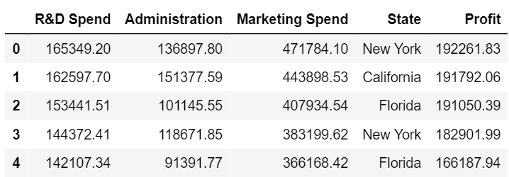
df.head()

# split the dataframe into dependent and independent variables.
x = df[['R&D Spend', 'Administration', 'Marketing Spend', 'State']]
y = df['Profit']
x.head()
y.head()

# since the state is a string datatype column we need to encode it.
x = pd.get_dummies(x)
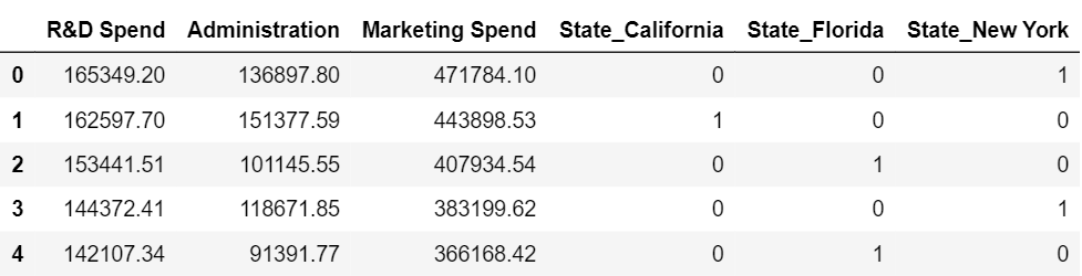
x.head()

Dataset

The set of independent variables after encoding the state column

Step 2 : Splitting the data into training and testing set and making predictions

x_train, x_test, y_train, y_test = train_test_split(
        x, y, test_size = 0.3, random_state = 0)
from sklearn.linear_model import LinearRegression
lm = LinearRegression()
lm.fit(x_train, y_train)
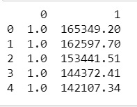
pred = lm.predict(x_test)

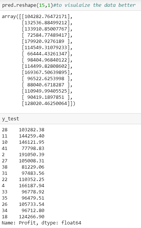
We can see that our predictions our close enough to the test set but how do we find the most important factor contributing to the profit.
Here is a solution for that.
We know that the equation of a multiple linear regression line is given by y=b1+b2*x+b3*x’+b4*x”+…….
where b1, b2, b3, … are the coefficients and x, x’, x” are all independent variables.
Since we don’t have any ‘x’ for the first coefficient we assume it can be written as a product of b and 1 and hence we append a column of ones. There are libraries that take care of it but since we are using the stats model library we need to explicitly add the column.
Step 3 : Using the backward elimination technique

import statsmodels.regression.linear_model as sm
# add a column of ones as integer data type
x = np.append(arr = np.ones((50, 1)).astype(int),
              values = x, axis = 1)
# choose a Significance level usually 0.05, if p>0.05
#  for the highest values parameter, remove that value
x_opt = x[:, [0, 1, 2, 3, 4, 5]]
ols = sm.OLS(endog = y, exog = x_opt).fit()
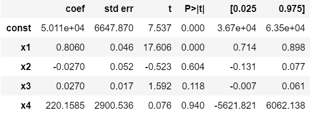
ols.summary()

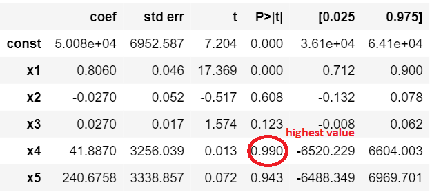
This figure shows the highest valued parameter

And now we follow the steps of the backward elimination and start eliminating unnecessary parameters.

# remove the 4th column as it has the highest value
x_opt = x[:, [0, 1, 2, 3, 5]]
ols = sm.OLS(endog = y, exog = x_opt).fit()
ols.summary()

# remove the 5th column as it has the highest value
x_opt = x[:, [0, 1, 2, 3]]
ols = sm.OLS(endog = y, exog = x_opt).fit()
ols.summary()

# remove the 3rd column as it has the highest value
x_opt = x[:, [0, 1, 2]]
ols = sm.OLS(endog = y, exog = x_opt).fit()
ols.summary()

# remove the 2nd column as it has the highest value
x_opt = x[:, [0, 1]]
ols = sm.OLS(endog = y, exog = x_opt).fit()
ols.summary()

Summary after removing the first unnecessary parameter.

So if we continue the process we see that we are left with only one column at the end and that is the R&D spent.We can conclude that the company which has maximum expenditure on the R&D makes the highest profit.

With this, we have solved the problem statement of finding the company for collaboration. Now let us have a brief look at the parameters of the OLS summary.

• R square – It tells about the goodness of the fit. It ranges between 0 and 1. The closer the value to 1, the better it is. It explains the extent of variation of the dependent variables in the model. However, it is biased in a way that it never decreases(even on adding variables).
• Adj Rsquare – This parameter has a penalising factor(the no. of regressors) and it always decreases or stays identical to the previous value as the number of independent variables increases. If its value keeps increasing on removing the unnecessary parameters go ahead with the model or stop and revert.
• F statistic – It is used to compare two variances and is always greater than 0. It is formulated as v1²/v2². In regression, it is the ratio of the explained to the unexplained variance of the model.
• AIC and BIC – AIC stands for Akaike’s information criterion and BIC stands for Bayesian information criterion Both these parameters depend on the likelihood function L.
• Skew – Informs about the data symmetry about the mean.
• Kurtosis – It measures the shape of the distribution i.e.the amount of data close to the mean than far away from the mean.
• Omnibus – D’Angostino’s test. It provides a combined statistical test for the presence of skewness and kurtosis.
• Log-likelihood – It is the log of the likelihood function.


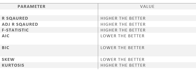
This image shows the preferred relative values of the parameters.
References:- Machine Learning course by Kirill Eremenko and Hadelin de Ponteves.