Linear Separability with Python

Linear Separability refers to the data points in binary classification problems which can be separated using linear decision boundary. if the data points can be separated using a line, linear function, or flat hyperplane are considered linearly separable.

• Linear separability is an important concept in neural networks. If the separate points in n-dimensional space follows  then it is said linearly separable
• For two-dimensional inputs, if there exists a line (whose equation is  ) that separates all samples of one class from the other class, then an appropriate perception can be derived from the equation of the separating line. such classification problems are called “Linear separable” i.e, separating by a linear combination of i/p.
• The logical AND gate example shown below illustrates a two-dimensional example of a linearly separable problem. 

Linear Separability as Mathematics:

Linear separability is introduced in the context of linear algebra and optimization theory. It speaks of the capacity of a hyperplane to divide two classes of data points in a high-dimensional space.

Let’s use the example of a set of data points in a p-dimensional space, where p is the number of features or variables that each point has to characterize it. 

A linear function   can be used to represent the hyperplane mathematically, where  are the features of the data point,   are corresponding weights. so that we can separate two different categories with a straight line and can represent them on the graph then we will say it is linearly separable the condition is only that it should be in the form y = ax + b form is the power of x should be 1 only then we can separate them linearly. 

   Since many classification techniques depend on the assumption of linear separability assumptions, linear separability is a key idea in machine learning. 

Methods for checking linear separability:

1. Visual Inspection: If a distinct straight line or plane divides the various groups, it can be visually examined by plotting the data points in a 2D or 3D space. The data may be linearly separable if such a boundary can be seen.
2. Perceptron Learning Algorithm: This binary linear classifier divides the input into two classes by learning a separating hyperplane iteratively. The data are linearly separable if the method finds a separating hyperplane and converges. If not, it is not.
3. Support vector machines: SVMs are a well-liked classification technique that can handle data that can be separated linearly. To optimize the margin between the two classes, they identify the separating hyperplane. The data can be linearly separated if the margin is bigger than zero.
4. Kernel methods: The data can be transformed into a higher-dimensional space using this family of techniques, where it might then be linearly separable. The original data is also linearly separable if the converted data is linearly separable.
5. Quadratic programming: Finding the separation hyperplane that reduces the classification error can be done using quadratic programming. If a solution is found, the data can be separated linearly.

In the real world, data points are frequently not perfectly linearly separable, hence Sometimes we use more advanced techniques to make the data points linearly separable.

Methods for converting Non-linear data into linear data:

Many techniques can be used to transform non-linearly separable data into linearly separable data. If the samples are not linearly separable,i.e no straight line can separate samples belonging to two classes, then there can not be any simple perception that archives the classification task. 

Here are a few typical strategies:

• Polynomial features: Converting non-linearly separable data into linearly separable data is simple when polynomial features are added. The decision boundary can be made more flexible and non-linear by including higher-order polynomial components, and the data may become linearly separable in the altered feature space.
• Kernel methods: The data can be linearly separable in a higher-dimensional space using kernel methods, which can translate the data into that space. Combining kernel approaches with support vector machines (SVMs), which can learn a linear decision boundary in the converted space.
• Neural networks: Neural networks are effective models that can learn intricate non-linear input–output mappings. We can learn a non-linear decision boundary that can categorize the data by using the more hidden layers in the neural network to train on non-linearly separable data.
• Manifold Learning: Finding the underlying structure of non-linearly separable data can be done via manifold learning, a sort of unsupervised learning. It might be possible to change the data into a higher-dimensional space where it is linearly separable by identifying the manifold on which it resides.

Checking Linear separability

• Import the necessary libraries
• Define custom dataset
• Build and train the linear model
• predict from new input

Python3

from sklearn import svm
import numpy as np

# Making dataset
X = np.array([[1, 2], [2, 3], [3, 1], [4, 3]])
Y = np.array([0, 0, 1, 1])

# Now lets train svm model
model = svm.SVC(kernel='linear')
model.fit(X, Y)

# Lets predict for new input
n_data = np.array([[5, 2], [2, 1]])
pred = model.predict(n_data)
print(pred)

Output : 

[1 0] 

Let’s plot the decision boundary for this

Python3

import matplotlib.pyplot as plt

# lets plot decision boundary for this
w = model.coef_[0]
b = model.intercept_[0]
x = np.linspace(1, 4)
y = -(w[0] / w[1]) * x - b / w[1]
plt.plot(x, y, 'k-')

# plot data points
plt.scatter(X[:, 0], X[:, 1], c=Y)
plt.xlabel('Feature 1')
plt.ylabel('Feature 2')
plt.show()

Output : 

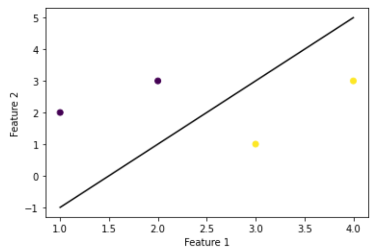
The plot of the decision boundary

 Convert Non-separable data to separable:

• Import the necessary libraries
• Create the non-linear dataset
• plot the dataset using matplotlib

Python3

from sklearn.datasets import make_circles
from sklearn.svm import SVC
import matplotlib.pyplot as plt
import numpy as np

# first lets create non-linear dataset
x_val, y_val = make_circles(n_samples=50, factor=0.5)

# Now lets plot and see our dataset
plt.scatter(x_val[:, 0], x_val[:, 1], c=y_val, cmap='plasma')
plt.show()

Output :

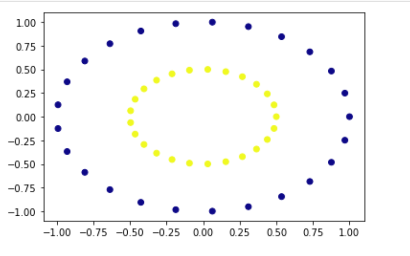
Non-Linearly Separable data

Apply kernel trick to map data into higher-dimensional space

• apply kernel trick to map data into higher-dimensional space.
• Now fit SVM on mapped data
• Plot decision boundary in mapped space
• plot mapped data

Python3

# apply kernel trick to map data into higher-dimensional space
x_new = np.vstack((x_val[:, 0]**2, x_val[:, 1]**2)).T

# Now fit SVM on mapped data
svm = SVC(kernel='linear')
svm.fit(x_new, y_val)

# plot decision boundary in mapped space
w = svm.coef_
a = -w[0][0] / w[0][1]
x = np.linspace(0, 1)
y = a * x - (svm.intercept_[0]) / w[0][1]
plt.plot(x, y, 'k-')

# plot mapped data
plt.scatter(x_new[:, 0], x_new[:, 1], c=y_val, cmap='plasma')
plt.show()

Output:

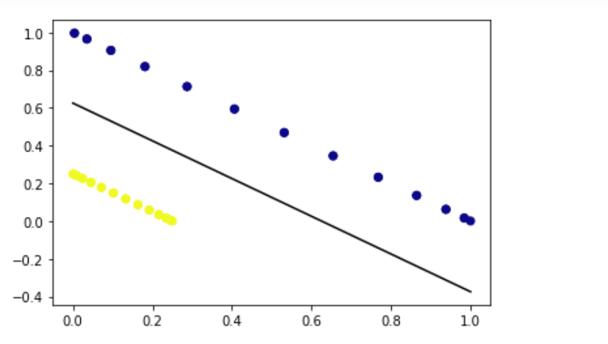
Separable data