Data Science – Solving Linear Equations with Python

A collection of equations with linear relationships between the variables is known as a system of linear equations. The objective is to identify the values of the variables that concurrently satisfy each equation, each of which is a linear constraint. By figuring out the system, we can learn how the variables interact and find hidden relationships or patterns. In disciplines including physics, engineering, economics, and computer science, it has a wide range of applications. Systems of linear equations can be solved quickly and with accurate results by using methods like Gaussian elimination, matrix factorization, inverse matrices and Lagrange function.

This is implemetations part of Data Science | Solving Linear Equations

Generalized linear equations

Generalized linear equations are represented as below:

Ax=b

Where,

• A is an mXn matrix
• x is nX1 variables or unknown terms
• b is the dependent variable mX1
• m & n are the numbers of equations and variables

In general, there are three cases one needs to understand: 

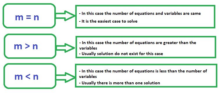
System of Linear Equations

Case A: m=n

Solution for the this type of linear equation can be find out using

Example 1

Consider the system of linear equation:

implementations

Python3

import numpy as np

# A 2 x 2 matrix
A = np.array([[2, 3],
              [5, 7]])
b =np.array([7, 10])

# Rank of matrix A
print("Rank of the matrix is:", np.linalg.matrix_rank(A))
# Inverse of matrix A
print("Inverse of A:\n", np.linalg.inv(A))

# Matrix equation solution
print("Solution of linear equations:\n", np.linalg.solve(A, b))

Output:

Rank of the matrix is: 2
Inverse of A:
[[-7.  3.]
[ 5. -2.]]
Solution of linear equations:
[-19.  15.]
array([-19.,  15.])

Example 2:

Consider the system of linear equation:

implementations

Python3

import numpy as np

# A 2 x 2 matrix
A = np.array([[2, 3],
              [4, 6]])
b =np.array([5, 10])

# Solution
def solution(A,b):
    if np.linalg.det(A) !=0:
        inv = np.linalg.inv(A)
        sol = inv@b
        return sol
    else:
        return 'infinite solution'

solution(A,b)

Output:

'infinite solution'

Case B: m>n

Solution for the this type of linear equation can be find out using

Example 1:

Consider the system of linear equation:

Implementations

Python3

import numpy as np

# A 2 x 2 matrix
A = np.array([[1, 2],
              [3, 7],
              [4,9]])
b =np.array([5, 10, 15])


# Solution
def solution(A,b):
    A_trans = A.T
    sol = np.linalg.inv(A_trans@A)@A_trans@b
    return sol

solution(A,b)

Output:

array([15., -5.])

Check the solutions

Python3

# Ax=b
A@solution(A,b)

Output:

array([ 5., 10., 15.])

Example 2:

Consider the system of linear equation:

Implementations

Python3

import numpy as np

# A 2 x 2 matrix
A = np.array([[1, 3],
              [3, 8],
              [4, 10]])
b =np.array([5, 10,15])


# Solution
def solution(A,b):
    A_trans = A.T
    sol = np.linalg.inv(A_trans@A)@A_trans@b
    return sol

solution(A,b)

Output:

array([2.22222222, 0.55555556])

Check the solutions

Python3

# Ax=b
A@solution(A,b)

Output:

array([ 3.88888889, 11.11111111, 14.44444444])

Case C: m < n

Solution for the this type of linear equation can be find out using

Example C.1:

Consider the system of linear equation:

Implementations

Python3

import numpy as np

# A 2 x 2 matrix
A = np.array([[1, 2, 3],
              [3, 4, 5]])

b =np.array([20,38])

# Solution x = A^T(AA^T)^(-1)b
def solution(A,b):
    sol = A.T @ np.linalg.pinv(A@A.T)@b
    return sol

solution(A,b)

Output:

array([2., 3., 4.])

Check the solutions

Python3

# Ax=b
A@solution(A,b)

Output:

array([20., 38.])

Example C.2:

Consider the system of linear equation:

Implementations

Python3

import numpy as np

# A 2 x 2 matrix
A = np.array([[1, 2, 5],
              [3, 5, 7]])

b =np.array([23,35])

# Solution x = A^T(AA^T)^(-1)b
def solution(A,b):
    sol = A.T @ np.linalg.pinv(A@A.T)@b
    return sol

solution(A,b)

Output:

array([0.36021505, 1.01075269, 4.12365591])

Check the solutions

Python3

# Ax=b
A@solution(A,b)

Output:

array([23., 35.])