Introduction to Tidy Data in R

Tidy data is a data science and analysis notion that entails arranging data in a systematic and consistent manner, making it easier to work with and analyze using tools such as R. Tidy data is a crucial component of Hadley Wickham’s data science methodology, which he popularized by creating the “tidyverse,” a set of R packages that contains tools for data modification, visualization, and analysis. We’ll look at the basics of tidy data in R and why it’s necessary for good data analysis in this introduction.

Tidy Data

Tidy data is a concept popularized by Hadley Wickham, the creator of the ggplot2 and dplyr packages in the R Programming Language. It’s an approach to structuring and organizing data in a consistent and standardized manner to simplify data manipulation, analysis, and visualization.

Tidy Data in R

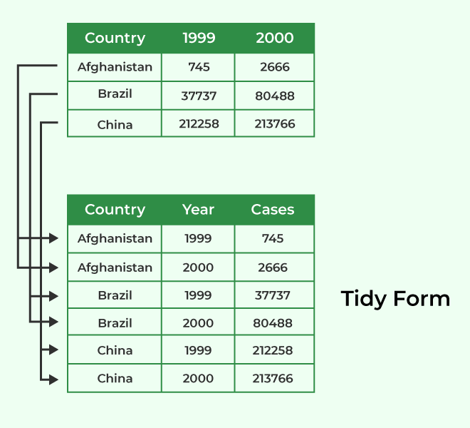
Tidy data follows a specific set of principles.

• Each Variable Forms a Column: In tidy data, each variable (or feature) in your dataset is represented by a separate column. This means that if you have multiple attributes or measurements, each attribute should have its own column.
• Each Observation Forms a Row: Each individual data point or observation corresponds to a single row in the dataset. Whether you’re dealing with measurements, events, or cases, each should be represented as a separate row.
• Each Type of Observational Unit Forms a Table: Tidy data encourages the organization of data into separate tables, where each table corresponds to a specific type of entity or observational unit. For example, if you’re dealing with sales data and customer data, you would have two separate tidy tables for these two distinct entities.
• Columns Contain Values: The cells within the dataset contain the actual values of the variables for each observation. In other words, the intersection of a row and column represents the value of a specific variable for a particular observation.
• Variables Have Descriptive Names: Column names should be descriptive and meaningful, making it easy to understand what each variable represents.
• Missing Values Are Handled Consistently: Tidy data provides a consistent approach to dealing with missing values, typically represented as NA or NULL in R.

By adhering to these principles, tidy data ensures that your datasets are structured in a way that simplifies data analysis and visualization. It makes it easier to use functions and tools from R packages like dplyr, ggplot2, tidyr, and others for data manipulation and exploration.

Advantages of Tidy Data

1. Facilitates data exploration: Tidy data structures make it easier to explore and understand your data.
2. Simplifies data transformation: Many R packages, like dplyr and tidyr, are designed to work seamlessly with tidy data, simplifying data transformation tasks.
3. Enhances data visualization: Tidy data works well with data visualization libraries like ggplot2, making it easier to create informative plots.
4. Promotes reproducibility: Tidy data helps in creating more reproducible workflows because data manipulation steps are more straightforward and documented.

Difference between tidy data and normal data

The term “tidy data” refers to a specific format or organization of data, while “normal data” is a more general term and does not refer to any specific data format. Let’s clarify the differences between these two concepts.

Normal (Untidy) Data

In this example, we have a dataset where different attributes (e.g., “Name,” “Age,” “City”) are stored in separate columns, and each row represents an individual’s information.

R

# Create a normal (untidy) data frame
normal_data <- data.frame(
  Name = c("Alice", "Bob", "Charlie"),
  Age = c(25, 30, 28),
  City = c("New York", "Los Angeles", "Chicago")
)

# Display the normal data
print(normal_data)

Output:

     Name Age        City
1   Alice  25    New York
2     Bob  30 Los Angeles
3 Charlie  28     Chicago

In this representation, each variable (Name, Age, City) has its own column, and each row corresponds to a different individual. This format is not considered tidy because each variable should be in a single column.

Tidy Data

In tidy data, each variable is stored in its own column, and each row represents a single observation or data point. To transform the normal data into tidy data, we can use the gather() function from the tidyr package.

R

# Load the tidyr package
library(tidyr)

# Convert the normal data to tidy format using gather()
tidy_data <- gather(normal_data, key = "Variable", value = "Value", -Name)

# Display the tidy data
print(tidy_data)

Output:

     Name Variable       Value
1   Alice      Age          25
2     Bob      Age          30
3 Charlie      Age          28
4   Alice     City    New York
5     Bob     City Los Angeles
6 Charlie     City     Chicago

In the tidy data representation, we have only three columns: “Name,” “Variable” (which stores the variable names), and “Value” (which stores the corresponding values). Each row represents a single observation, and the data is now structured in a way that follows the principles of tidy data.

Certainly, here’s another example that demonstrates the difference between normal (untidy) data and tidy data using R. In this example, we’ll work with a dataset related to sales data for different products.

Another example to demonstrate the Normal Data and Tidy Data

Normal (Untidy) Data:

In this normal (untidy) data representation, we have different products as columns, and each row represents a sales record for a specific date.

R

# Create a normal (untidy) data frame
normal_data <- data.frame(
  Date = as.Date(c("2023-01-01", "2023-01-02", "2023-01-03")),
  ProductA = c(100, 120, 90),
  ProductB = c(80, 75, 95),
  ProductC = c(60, 70, 80)
)

# Display the normal data
print(normal_data)

Output:

        Date ProductA ProductB ProductC
1 2023-01-01      100       80       60
2 2023-01-02      120       75       70
3 2023-01-03       90       95       80

In this representation, each product (ProductA, ProductB, ProductC) has its own column, and each row corresponds to sales data for a specific date. This format is not considered tidy because each variable (product) should be in a single column.

Tidy Data

In tidy data, we’ll restructure the data so that it follows the principles of tidy data. Each variable (product) will be stored in its own column, and each row will represent a single sales record.

R

# Load the tidyr package
library(tidyr)

# Convert the normal data to tidy format using gather()
tidy_data <- gather(normal_data, key = "Product", value = "Sales", -Date)

# Display the tidy data
print(tidy_data)

Output:

      Date  Product Sales
1 2023-01-01 ProductA   100
2 2023-01-02 ProductA   120
3 2023-01-03 ProductA    90
4 2023-01-01 ProductB    80
5 2023-01-02 ProductB    75
6 2023-01-03 ProductB    95
7 2023-01-01 ProductC    60
8 2023-01-02 ProductC    70
9 2023-01-03 ProductC    80

In the tidy data representation, we have three columns: “Date,” “Product” (which stores the product names), and “Sales” (which stores the corresponding sales values). Each row represents a single sales record, and the data is now structured in a way that follows the principles of tidy data.

Conclusion

The key difference between tidy data and normal data lies in their organization and adherence to specific principles. Tidy data is structured according to principles that facilitate data analysis, while normal data can take on various formats that may require additional effort to prepare for analysis. Tidy data is particularly useful when working with tools and packages designed to operate on well-structured data, such as those in the tidyverse ecosystem in R.