How to Implement Adam Gradient Descent from Scratch using Python?

Grade descent is an extensively used optimization algorithm in machine literacy and deep literacy. It’s used to minimize the cost or loss function of a model by iteratively confirming the model’s parameters grounded on the slants of the cost function with respect to those parameters. One variant of gradient descent that has gained popularity is the Adam optimization algorithm. Adam combines the benefits of AdaGrad and RMSProp to achieve effective and adaptive learning rates.

Understanding the Adam Algorithm

Before going into the implementation, let’s have a brief overview of the Adam optimization algorithm. Adam stands for Adaptive Moment Estimation. It maintains two moving average variables: 

• v – For the first moment
• s – For the second moment

The algorithm computes an exponentially weighted average of the past gradients and their squared gradients. These moving averages are then used to update the model’s parameters.

The Adam algorithm consists of the following steps:

1. Initialize the Variables: The algorithm starts by initializing the moving average variables v and s as dictionaries to store the exponentially weighted averages of the gradients and squared gradients, respectively.
2. Compute Moving Averages: For each parameter of the model, the algorithm computes the moving average of the gradients by combining the current gradient with the previous moving average. It also computes the moving average of the squared gradients.
3. Bias Correction: To reduce bias during the initial iterations, Adam performs bias correction by dividing the moving averages by a correction factor.
4. Update Parameters: Finally, the algorithm updates the parameters of the model using the moving averages of the gradients and squared gradients.

Terminologies related to Adam’s Algorithm

1. Gradient Descent: An iterative optimization algorithm used to find the minimum of a function by iteratively adjusting the parameters in the direction of the steepest descent of the gradient.
2. Learning Rate: A hyperparameter that determines the step size at each iteration of gradient descent. It controls how much the parameters are updated based on the computed gradients.
3. Objective Function: The function that we aim to minimize or maximize. In the context of optimization, it is usually a cost function or a loss function.
4. Derivative: The derivative of a function represents its rate of change at a particular point. In the context of gradient descent, the derivative (or gradient) provides the direction and magnitude of the steepest ascent or descent.
5. Local Minimum: A point in the optimization landscape where the objective function has the lowest value in the vicinity. It may not be the global minimum, which is the absolute lowest point in the entire optimization landscape.
6. Global Minimum: The lowest point in the entire optimization landscape, indicating the optimal solution to the problem.
7. Momentum: In the context of optimization algorithms, momentum refers to the inclusion of past gradients to determine the current update. It helps accelerate convergence and overcome local optima.
8. Adam (Adaptive Moment Estimation): An optimization algorithm that extends gradient descent by utilizing adaptive learning rates and momentum. It maintains a running average of past gradients and squared gradients to compute adaptive learning rates for each parameter.
9. Beta1 and Beta2: Hyperparameters in the Adam algorithm that control the exponential decay rates for the estimation of the first and second moments of the gradients, respectively. Beta1 controls the momentum-like effect, while Beta2 controls the influence of the squared gradients.
10. Epsilon (eps): A small constant added to the denominator in the Adam algorithm to prevent division by zero and ensure numerical stability.

Now that we have a basic understanding of the Adam algorithm, let’s proceed with implementing it from scratch in Python. The algorithm gets its name from “Adaptive Moment Estimation” as it calculates adaptive learning rates for each parameter by estimating the first and second moments of the gradients.

Implementing Adam Gradient Descent

We start by importing the necessary libraries. In this implementation, we only need the NumPy library for mathematical operations. The initialize_adam function initializes the moving average variables v and s as dictionaries based on the parameters of the model. It takes the parameters dictionary as input, which contains the weights and biases of the model.

v = 0 (Initialize first moment vector)
s = 0 (Initialize second moment vector)
t = 0 (Initialize time step)

Python3

def initialize_adam(parameters):
    L = len(parameters) // 2
    v = {}
    s = {}

    for l in range(L):
        v["dW" + str(l+1)] = np.zeros_like(parameters["W" + str(l+1)])
        v["db" + str(l+1)] = np.zeros_like(parameters["b" + str(l+1)])
        s["dW" + str(l+1)] = np.zeros_like(parameters["W" + str(l+1)])
        s["db" + str(l+1)] = np.zeros_like(parameters["b" + str(l+1)])

    return v, s

The function initializes the moving average variables for both weights (dW) and biases (db) of each layer in the model. It returns the initialized v and s dictionaries.

In above code,

initialize_adam(): This function is responsible for initializing the moments s and v used in the Adam algorithm. The moments are initialized with zero values to ensure a proper start for the optimization process. By initializing these moments, Adam keeps track of the first and second moments of the gradients for each parameter, which helps in adapting the learning rate during optimization.

Mathematical Intuition Behind Adam’s Gradient Descent

The update_parameters_with_adam function performs the Adam gradient descent update for the parameters of the model. It takes the parameters dictionary, gradients grads, moving averages v and s, iteration number t, learning rate learning_rate, and hyperparameters beta1, beta2, and epsilon as inputs.

\begin{aligned} m_t &= \beta_1 * m_{t-1} + \left(1 – \beta_1 \right ) * \nabla w_t \\v_t &= \beta_2 * v_{t-1} + \left(1 – \beta_2 \right ) * \left(\nabla w_t \right )^2 \\\hat{m_t} &= \frac{m_t}{1 – {\beta_1}^t}\\ \hat{v_t} &= \frac{v_t}{1 – {\beta_2}^t}\\ w_{t + 1} &= w_t – \frac{\eta}{\sqrt{\hat{v_t} + \epsilon}} * \hat{m_t} \end{aligned} 

where:

• w_t is the parameters or weights of the model.
• learning_rate(eta) is the step size or the learning rate hyperparameter.
• beta1 and beta2 are the decay rates for the first and second moments, respectively.
• s is the first-moment estimate (mean) of the gradients.
• v is the second-moment estimate (uncentered variance) of the gradients.
• t is the current iteration.
• epsilon is a small constant to ensure numerical stability.

Python3

def update_parameters_with_adam(parameters, grads,
                                v, s, t, learning_rate=0.01,
                                beta1=0.9, beta2=0.999,
                                epsilon=1e-8):
    L = len(parameters) // 2
    v_corrected = {}
    s_corrected = {}

    for l in range(L):
        # Compute moving average of the gradients
        v["dW" + str(l+1)] = beta1 * v["dW" + str(l+1)] + \
            (1 - beta1) * grads["dW" + str(l+1)]
        v["db" + str(l+1)] = beta1 * v["db" + str(l+1)] + \
            (1 - beta1) * grads["db" + str(l+1)]

        # Compute bias-corrected first moment estimate
        v_corrected["dW" + str(l+1)] = v["dW" + str(l+1)] / (1 - beta1**t)
        v_corrected["db" + str(l+1)] = v["db" + str(l+1)] / (1 - beta1**t)

        # Compute moving average of the squared gradients
        s["dW" + str(l+1)] = beta2 * s["dW" + str(l+1)] + \
            (1 - beta2) * (grads["dW" + str(l+1)]**2)
        s["db" + str(l+1)] = beta2 * s["db" + str(l+1)] + \
            (1 - beta2) * (grads["db" + str(l+1)]**2)

        # Compute bias-corrected second raw moment estimate
        s_corrected["dW" + str(l+1)] = s["dW" + str(l+1)] / (1 - beta2**t)
        s_corrected["db" + str(l+1)] = s["db" + str(l+1)] / (1 - beta2**t)

        # Update parameters
        parameters["W" + str(l+1)] = parameters["W" + str(l+1)]\
        - learning_rate * (
            v_corrected["dW" + str(l+1)] / \
          (np.sqrt(s_corrected["dW" + str(l+1)]) + epsilon))

update_parameters_with_adam(): This function plays a crucial role in updating the parameters based on the computed gradients and the Adam moments. It takes the current parameters, gradients, moments s and v, and other hyperparameters of the algorithm as inputs. The function applies the Adam update rule, incorporating the bias-corrected moments, learning rate, and other factors to ensure accurate parameter updates. The updated parameters, along with the updated moments, are returned for the next iteration. This update process helps the algorithm converge faster and more effectively by adjusting the learning rate for each parameter individually.

The function iterates through each layer of the model and performs the following steps:

• Compute the moving average of the gradients using the beta1 hyperparameter.
• Compute the bias-corrected first-moment estimate.
• Compute the moving average of the squared gradients using the beta2 hyperparameter.
• Compute the bias-corrected second raw moment estimate.
• Update the parameters using the computed moving averages.

This function updates the weights and biases of each layer based on the Adam optimization algorithm. Now, implementing the Adam gradient descent optimization algorithm:

Python3

import numpy as np

# Objective function
def objective(x, y):
    return x ** 2.0 + y ** 2.0

# Derivative of the objective function
def derivative(x, y):
    return np.array([2.0 * x, 2.0 * y])

# Initialize Adam moments
def initialize_adam():
    s = np.zeros(2)
    v = np.zeros(2)
    return m, v

# Update parameters using Adam
def update_parameters_with_adam(x, grads, s, v,
                                t, learning_rate=0.01,
                                beta1=0.9, beta2=0.999,
                                epsilon=1e-8):
    s = beta1 * s + (1.0 - beta1) * grads
    v = beta2 * v + (1.0 - beta2) * grads ** 2
    s_hat = m / (1.0 - beta1 ** (t + 1))
    v_hat = v / (1.0 - beta2 ** (t + 1))
    x = x - learning_rate * s_hat / (np.sqrt(v_hat) + epsilon)
    return x, s, v

# Adam optimization algorithm
def adam(objective, derivative, bounds,
         n_iter, alpha, beta1, beta2, eps=1e-8):
    # Generate an initial point
    x = bounds[:, 0] + np.random.rand(len(bounds))\
    * (bounds[:, 1] - bounds[:, 0])
    score = objective(x[0], x[1])

    # Initialize Adam moments
    m, v = initialize_adam()

    # Run the gradient descent updates
    for t in range(n_iter):
        # Calculate gradient g(t)
        g = derivative(x[0], x[1])

        # Update parameters using Adam
        x, s, v = update_parameters_with_adam(x, g, s,
                                              v, t, alpha,
                                              beta1, beta2,
                                              eps)

        # Evaluate candidate point
        score = objective(x[0], x[1])

        # Report progress
        print('>%d f(%s) = %.5f' % (t, x, score))

    return [x, score]

# Set the random seed
np.random.seed(1)

# Define the range for input
bounds = np.array([[-1.0, 1.0], [-1.0, 1.0]])

# Define the total number of iterations
n_iter = 60

# Set the step size
alpha = 0.02

# Set the factor for average gradient
beta1 = 0.8

# Set the factor for average squared gradient
beta2 = 0.999

# Perform the gradient descent search with Adam
best, score = adam(objective, derivative,
                   bounds, n_iter, alpha,
                   beta1, beta2)
print('Done!')
print('f(%s) = %f' % (best, score))

Output:

>0 f([-0.14595599  0.42064899]) = 0.19825
>1 f([-0.12613855  0.40070573]) = 0.17648
>2 f([-0.10665938  0.3808601 ]) = 0.15643
>3 f([-0.08770234  0.3611548 ]) = 0.13812
>4 f([-0.06947941  0.34163405]) = 0.12154
>5 f([-0.05222756  0.32234308]) = 0.10663
>6 f([-0.03620086  0.30332769]) = 0.09332
>7 f([-0.02165679  0.28463383]) = 0.08149
>8 f([-0.00883663  0.26630707]) = 0.07100
>9 f([0.00205801 0.24839209]) = 0.06170
>10 f([0.01088844 0.23093228]) = 0.05345
>11 f([0.01759677 0.2139692 ]) = 0.04609
>12 f([0.02221425 0.19754214]) = 0.03952
>13 f([0.02485859 0.18168769]) = 0.03363
>14 f([0.02572196 0.16643933]) = 0.02836
>15 f([0.02505339 0.15182705]) = 0.02368
>16 f([0.02313917 0.13787701]) = 0.01955
>17 f([0.02028406 0.12461125]) = 0.01594
>18 f([0.01679451 0.11204744]) = 0.01284
>19 f([0.01296436 0.10019867]) = 0.01021
>20 f([0.00906264 0.08907337]) = 0.00802
>21 f([0.00532366 0.07867522]) = 0.00622
>22 f([0.00193919 0.06900318]) = 0.00477
>23 f([-0.00094677  0.06005154]) = 0.00361
>24 f([-0.00324034  0.05181012]) = 0.00269
>25 f([-0.00489722  0.04426444]) = 0.00198
>26 f([-0.00591902  0.03739604]) = 0.00143
>27 f([-0.00634719  0.0311828 ]) = 0.00101
>28 f([-0.00625503  0.02559933]) = 0.00069
>29 f([-0.00573849  0.02061737]) = 0.00046
>30 f([-0.00490679  0.01620624]) = 0.00029
>31 f([-0.00387317  0.01233332]) = 0.00017
>32 f([-0.00274675  0.00896449]) = 0.00009
>33 f([-0.00162559  0.00606458]) = 0.00004
>34 f([-0.00059149  0.00359785]) = 0.00001
>35 f([0.0002934  0.00152838]) = 0.00000
>36 f([ 0.00098821 -0.00017954]) = 0.00000
>37 f([ 0.00147307 -0.00156101]) = 0.00000
>38 f([ 0.00174746 -0.00265025]) = 0.00001
>39 f([ 0.00182724 -0.00348028]) = 0.00002
>40 f([ 0.00174089 -0.00408267]) = 0.00002
>41 f([ 0.00152536 -0.00448737]) = 0.00002
>42 f([ 0.00122173 -0.00472254]) = 0.00002
>43 f([ 0.00087133 -0.00481438]) = 0.00002
>44 f([ 0.00051228 -0.00478712]) = 0.00002
>45 f([ 0.00017692 -0.00466292]) = 0.00002
>46 f([-0.00011001 -0.00446188]) = 0.00002
>47 f([-0.00033219 -0.004202  ]) = 0.00002
>48 f([-0.00048176 -0.00389929]) = 0.00002
>49 f([-0.00055861 -0.00356777]) = 0.00001
>50 f([-0.00056912 -0.00321961]) = 0.00001
>51 f([-0.00052452 -0.00286514]) = 0.00001
>52 f([-0.00043908 -0.00251304]) = 0.00001
>53 f([-0.0003283  -0.00217044]) = 0.00000
>54 f([-0.00020731 -0.00184302]) = 0.00000
>55 f([-8.95352320e-05 -1.53514076e-03]) = 0.00000
>56 f([ 1.43050285e-05 -1.25002847e-03]) = 0.00000
>57 f([ 9.67123406e-05 -9.89850279e-04]) = 0.00000
>58 f([ 0.00015359 -0.00075587]) = 0.00000
>59 f([ 0.00018407 -0.00054858]) = 0.00000
Done!
f([ 0.00018407 -0.00054858]) = 0.000000

Visualization of Adam

To visualize the optimization process using the Adam algorithm, we can plot the trajectory of the candidate points as they move toward the minimum of the objective function. Here’s an example of how you can visualize the optimization process using Matplotlib:

Python3

import numpy as np
import matplotlib.pyplot as plt
from mpl_toolkits.mplot3d import Axes3D

# Objective function
def objective(x, y):
    return x ** 2.0 + y ** 2.0

# Derivative of the objective function
def derivative(x, y):
    return np.array([2.0 * x, 2.0 * y])

# Gradient descent algorithm with Adam
def adam(objective, derivative, bounds, n_iter,
         alpha, beta1, beta2, eps=1e-8):
    # Generate an initial point
    x = bounds[:, 0] + np.random.rand(len(bounds))\
    * (bounds[:, 1] - bounds[:, 0])
    scores = []
    trajectory = []

    # Initialize first and second moments
    m = np.zeros(bounds.shape[0])
    v = np.zeros(bounds.shape[0])

    # Run the gradient descent updates
    for t in range(n_iter):
        # Calculate gradient g(t)
        g = derivative(x[0], x[1])

        # Build a solution one variable at a time
        for i in range(x.shape[0]):
            # m(t) = beta1 * m(t-1) + (1 - beta1) * g(t)
            m[i] = beta1 * m[i] + (1.0 - beta1) * g[i]
            # v(t) = beta2 * v(t-1) + (1 - beta2) * g(t)^2
            v[i] = beta2 * v[i] + (1.0 - beta2) * g[i] ** 2
            # mhat(t) = m(t) / (1 - beta1(t))
            mhat = m[i] / (1.0 - beta1 ** (t + 1))
            # vhat(t) = v(t) / (1 - beta2(t))
            vhat = v[i] / (1.0 - beta2 ** (t + 1))
            # x(t) = x(t-1) - alpha * mhat(t) / (sqrt(vhat(t)) + eps)
            x[i] = x[i] - alpha * mhat / (np.sqrt(vhat) + eps)

        # Evaluate candidate point
        score = objective(x[0], x[1])
        scores.append(score)
        trajectory.append(x.copy())

    return x, scores, trajectory

# Define the range for input
bounds = np.array([[-1.0, 1.0], [-1.0, 1.0]])

# Define the total number of iterations
n_iter = 60

# Set the step size
alpha = 0.02

# Set the factor for average gradient
beta1 = 0.8

# Set the factor for average squared gradient
beta2 = 0.999

# Perform the gradient descent search with Adam
best, scores, trajectory = adam(objective, derivative,
                                bounds, n_iter, alpha,
                                beta1, beta2)

# Generate a grid of points for visualization
x = np.linspace(bounds[0, 0], bounds[0, 1], 100)
y = np.linspace(bounds[1, 0], bounds[1, 1], 100)
X, Y = np.meshgrid(x, y)
Z = objective(X, Y)

# Plot the optimization trajectory
fig = plt.figure()
ax = fig.add_subplot(111, projection='3d')
ax.plot_surface(X, Y, Z, cmap='viridis', alpha=0.5)
ax.scatter(best[0], best[1], objective(best[0], best[1]),
           color='red', label='Best')
ax.plot([point[0] for point in trajectory],
        [point[1] for point in trajectory], scores,
        color='blue', label='Trajectory')
ax.set_xlabel('X')
ax.set_ylabel('Y')
ax.set_zlabel('Objective')
ax.legend()

# Show the plot
plt.show()

Output:

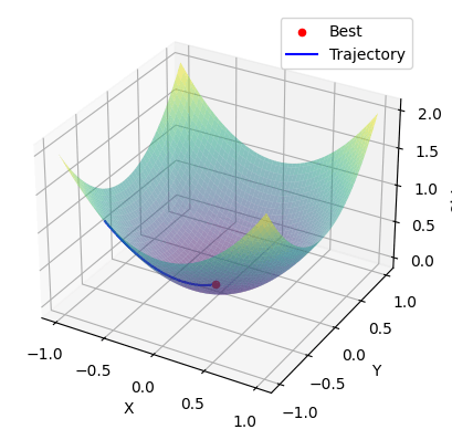
Global Minima Using Adam Optimization Algorithm

The above code generates a 3D plot of the objective function and overlays the optimization trajectory of the candidate points. The best solution found is shown as a red dot, and the trajectory is shown as a blue line connecting the candidate points.

Advantages of the Adam Algorithm

1. Effective Handling of Sparse Gradients: Adam performs well on datasets with sparse gradients, making it suitable for tasks involving noisy or irregularly sampled data.
2. Default Hyperparameter Values: Adam’s default hyperparameter values often yield good results across a wide range of problems, reducing the need for extensive hyperparameter tuning.
3. Computational Efficiency: Adam is computationally efficient, making it suitable for large-scale optimization tasks with a high-dimensional parameter space.
4. Memory Efficiency: Adam requires relatively low memory compared to some other optimization algorithms, making it memory-efficient, particularly when dealing with large datasets.
5. Suitable for Large Datasets: Adam is well-suited for optimization problems involving large datasets, as it efficiently updates the parameters based on the accumulated gradients.

Disadvantages of the Adam Algorithm

1. Convergence Issues in Certain Cases: Adam may not converge to an optimal solution in some cases, particularly in regions with complex or irregular geometry. This limitation has motivated the development of alternative variants such as AMSGrad.
2. Weight Decay Problem: Adam can suffer from a weight decay problem, where the weight decay term overly penalizes the parameters during optimization. This issue has been addressed in variations like AdamW, which incorporate additional techniques to mitigate the problem.
3. Continuous Algorithm Improvements: Recent advancements in optimization algorithms have demonstrated better performance and faster convergence rates compared to Adam, indicating that there are alternatives that may outperform it in certain scenarios.