Vectorization Of Gradient Descent

Last Updated : 24 Oct, 2020

In Machine Learning, Regression problems can be solved in the following ways:

1. Using Optimization Algorithms – Gradient Descent

Batch Gradient Descent.
Stochastic Gradient Descent.
Mini-Batch Gradient Descent
Other Advanced Optimization Algorithms like ( Conjugate Descent … )

2. Using the Normal Equation :

Using the concept of Linear Algebra.

Let’s consider the case for Batch Gradient Descent for Univariate Linear Regression Problem.

The cost function for this Regression Problem is :

$J(\Theta)=(1/2m)*\sum_{i=1}^m(h_{\theta}(x^i)-y^i)^2$

Goal:

$minimize_{\ \theta_{o},\theta_{1}}\ \ J({\theta})$

In order to solve this problem, we can either go for a Vectorized approach ( Using the concept of Linear Algebra ) or unvectorized approach (Using for-loop).

1. Unvectorized Approach:

Here in order to solve the below mentioned mathematical expressions, We use for loop.

The above mathematical expression is a part of Cost Function.

$\sum_{i=1}^m(h_{\theta}(x^i)-y^i)^2$

The above Mathematical Expression is the hypothesis.

$h_{\theta}=\theta_{0}x_{0}+\theta_{1}x_{1}+\theta_{2}x_{2}+... +\theta_{n}x_{n}\\ where,\\ h_{\theta}=hypothesis.\\$ Code: Python Implementation of Unvectorzed Grad

# Import required modules. 
from sklearn.datasets import make_regression 
import matplotlib.pyplot as plt 
import numpy as np 
import time 
   
# Create and plot the data set. 
x, y = make_regression(n_samples = 100, n_features = 1, 
                       n_informative = 1, noise = 10, random_state = 42) 
  
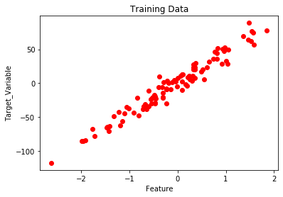
plt.scatter(x, y, c = 'red') 
plt.xlabel('Feature') 
plt.ylabel('Target_Variable') 
plt.title('Training Data') 
plt.show() 
  
# Convert y from 1d to 2d array. 
y = y.reshape(100, 1) 
   
# Number of Iterations for Gradient Descent 
num_iter = 1000
   
# Learning Rate 
alpha = 0.01
   
# Number of Training samples. 
m = len(x) 
   
# Initializing Theta. 
theta = np.zeros((2, 1),dtype = float) 
   
# Variables 
t0 = t1 = 0
Grad0 = Grad1 = 0
  
# Batch Gradient Descent. 
start_time = time.time() 
   
for i in range(num_iter): 
    # To find Gradient 0. 
    for j in range(m): 
        Grad0 = Grad0 + (theta[0] + theta[1] * x[j]) - (y[j]) 
      
    # To find Gradient 1. 
    for k in range(m): 
        Grad1 = Grad1 + ((theta[0] + theta[1] * x[k]) - (y[k])) * x[k] 
    t0 = theta[0] - (alpha * (1/m) * Grad0) 
    t1 = theta[1] - (alpha * (1/m) * Grad1) 
    theta[0] = t0 
    theta[1] = t1 
    Grad0 = Grad1 = 0
       
# Print the model parameters.     
print('model parameters:',theta,sep = '\n') 
   
# Print Time Take for Gradient Descent to Run. 
print('Time Taken For Gradient Descent in Sec:',time.time()- start_time) 
  
# Prediction on the same training set. 
h = [] 
for i in range(m): 
    h.append(theta[0] + theta[1] * x[i]) 
       
# Plot the output. 
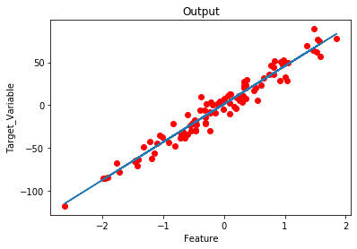
plt.plot(x,h) 
plt.scatter(x,y,c = 'red') 
plt.xlabel('Feature') 
plt.ylabel('Target_Variable') 
plt.title('Output')

Output:

model parameters:
[[ 1.15857049]
 [44.42210912]]
 
Time Taken For Gradient Descent in Sec: 2.482538938522339

2. Vectorized Approach:

Here in order to solve the below mentioned mathematical expressions, We use Matrix and Vectors (Linear Algebra).

The above mathematical expression is a part of Cost Function.

$\sum_{i=1}^m(h_{\theta}(x^i)-y^i)^2$

The above Mathematical Expression is the hypothesis.

$h_{\theta}=\theta^T.X\\ where,\\ h_{\theta}=hypothesis.\\ \theta= \begin{bmatrix} \theta_{0} \\ \theta_{1}\\ \theta_{2}\\ \theta_{3}\\ .\\ .\\ \theta_{n}\\ \end{bmatrix} X= \begin{bmatrix} {x_{0}} \\ {x_{1}}\\ {x_{2}}\\ {x_{3}}\\ .\\ .\\ {x_{n}}\\ \end{bmatrix}\\$

Batch Gradient Descent :

$Loop\ until\ converge\{\\ \ \theta_{j}:=\theta_{j}-(1/m)*(\alpha)*\frac{\partial J(\theta)}{\partial \theta_{j}} \\ \}\\ Let, \ Gradients=\frac{\partial J(\theta)}{\partial \theta_{j}}$

Concept To Find Gradients Using Matrix Operations:

$X\_New= \begin{bmatrix} {x_{0}^1} & {x_{1}^1} \\ {x_{0}^2} & {x_{1}^2}\\ {x_{0}^3} & {x_{1}^3}\\ {x_{0}^4} & {x_{1}^4}\\ . & .\\ . & .\\ . & .\\ {x_{0}^m} & {x_{1}^m} \end{bmatrix}_{m X 2} \theta= \begin{bmatrix} \theta_{0} \\ \theta_{1}\\ \end{bmatrix}_{2X1}\\ where,\\ \x_{0}^i=1\\$ $H(\theta)=X\_New\ .\ \theta\\ H(\theta)= \begin{bmatrix} {\Theta_{0}}{x_{0}^1}+{\Theta_{1}}{x_{1}^1} \\ {\Theta_{0}}{x_{0}^2}+{\Theta_{1}}{x_{1}^2}\\ {\Theta_{0}}{x_{0}^3}+{\Theta_{1}}{x_{1}^3}\\ {\Theta_{0}}{x_{0}^4}+{\Theta_{1}}{x_{1}^4}\\ .\\ .\\ . \\ {\Theta_{0}}{x_{0}^m}+{\Theta_{1}}{x_{1}^m} \end{bmatrix}_{mX1} And\ \ \ Y= \begin{bmatrix} {y^1}\\ {y^2}\\ {y^3}\\ .\\ .\\ .\\ {y^m} \end{bmatrix}_{mX1}\\$ $H(\theta)-Y= \begin{bmatrix} {\Theta_{0}}{x_{0}^1}+{\Theta_{1}}{x_{1}^1} -y^1\\ {\Theta_{0}}{x_{0}^2}+{\Theta_{1}}{x_{1}^2}-y^2\\ {\Theta_{0}}{x_{0}^3}+{\Theta_{1}}{x_{1}^3}-y^3\\ {\Theta_{0}}{x_{0}^4}+{\Theta_{1}}{x_{1}^4}-y^4\\ .\\ .\\ . \\ {\Theta_{0}}{x_{0}^m}+{\Theta_{1}}{x_{1}^m}-y^m \end{bmatrix}_{mX1} \\$ $X\_New^T= \begin{bmatrix} {x_{0}^1\ x_{0}^2\ x_{0}^3\ .\ .\ .\ x_{0}^m}\\ {x_{1}^1\ x_{1}^2\ x_{1}^3\ .\ .\ .\ x_{1}^m} \end{bmatrix}_{2Xm} \\$ $Gradients=X\_New\ . \ (H(\theta)-Y)\\ = \begin{bmatrix} {x_{0}^1(\Theta x_{0}^1+\Theta x_{1}^1-y^1)\ + \ x_{0}^2(\Theta x_{0}^2+\Theta x_{1}^2-y^2)\ + \ x_{0}^3(\Theta x_{0}^3+\Theta x_{1}^3-y^3)\ + . . .}\\ {x_{1}^1(\Theta x_{0}^1+\Theta x_{1}^1-y^1)\ + \ x_{1}^2(\Theta x_{0}^2+\Theta x_{1}^2-y^2)\ + \ x_{1}^3(\Theta x_{0}^3+\Theta x_{1}^3-y^3)\ + . . .}\\ \end{bmatrix}_{2X1}\\$ $Finally\ we\ can \ say,\\ \ \ \ Gradients=\frac{\partial J(\theta)}{\partial \theta_{j}}=X\_New^T.(X\_New.\theta-Y)$ Code: Python implementation of vectorized Gradient Descent approach

# Import required modules. 
from sklearn.datasets import make_regression 
import matplotlib.pyplot as plt 
import numpy as np 
import time 
   
# Create and plot the data set. 
x, y = make_regression(n_samples = 100, n_features = 1, 
                       n_informative = 1, noise = 10, random_state = 42) 
  
plt.scatter(x, y, c = 'red') 
plt.xlabel('Feature') 
plt.ylabel('Target_Variable') 
plt.title('Training Data') 
plt.show() 
  
  
# Adding x0=1 column to x array. 
X_New = np.array([np.ones(len(x)), x.flatten()]).T 
  
# Convert y from 1d to 2d array. 
y = y.reshape(100, 1) 
   
# Number of Iterations for Gradient Descent 
num_iter = 1000
   
# Learning Rate 
alpha = 0.01
   
# Number of Training samples. 
m = len(x) 
   
# Initializing Theta. 
theta = np.zeros((2, 1),dtype = float) 
   
# Batch-Gradient Descent. 
start_time = time.time() 
   
for i in range(num_iter): 
    gradients = X_New.T.dot(X_New.dot(theta)- y) 
    theta = theta - (1/m) * alpha * gradients 
   
# Print the model parameters.     
print('model parameters:',theta,sep = '\n') 
   
# Print Time Take for Gradient Descent to Run. 
print('Time Taken For Gradient Descent in Sec:',time.time() - start_time) 
  
# Hypothesis. 
h = X_New.dot(theta) # Prediction on training data itself. 
   
# Plot the Output. 
plt.scatter(x, y, c = 'red') 
plt.plot(x ,h) 
plt.xlabel('Feature') 
plt.ylabel('Target_Variable') 
plt.title('Output')

Output:

model parameters:
[[ 1.15857049]
 [44.42210912]]
 
Time Taken For Gradient Descent in Sec: 0.019551515579223633

Observations:

Implementing a vectorized approach decreases the time taken for execution of Gradient Descent( Efficient Code ).
Easy to debug.

Suggest improvement

Identifying handwritten digits using Logistic Regression in PyTorch

BeautifulSoup object - Python Beautifulsoup

Share your thoughts in the comments