Handling Missing Values in Time Series Data

Handling missing values in time series data in R is a crucial step in the data preprocessing phase. Time series data often contains gaps or missing observations due to various reasons such as sensor malfunctions, human errors, or other external factors. In R Programming Language dealing with missing values appropriately is essential to ensure the accuracy and reliability of analyses and models built on time series data. Here are some common strategies for handling missing values in time series data.

Understanding Missing Values in Time Series Data

In general Time Series data is a type of data where observations are collected over some time at successive intervals. Time series are used in various fields such as finance, engineering, and biological sciences, etc,

• Missing values will disrupt the order of the data which indirectly results in the inaccurate representation of trends and patterns over some time
• By Imputing missing values we can ensure the statistical analysis done on the Time Serial data is reliable based on the patterns we observed.
• Similar to other models handling missing values in the time series data improves the model performance.

In R Programming there are various ways to handle missing values of Time Series Data using functions that are present under the ZOO package.

It’s important to note that the choice of method depends on the nature of the data and the underlying reasons for missing values. A combination of methods or a systematic approach to evaluating different imputation strategies may be necessary to determine the most suitable approach for a given time series dataset. Additionally, care should be taken to assess the impact of missing value imputation on the validity of subsequent analyses and models.

Step 1: Load Necessary Libraries and Dataset

R

# Load necessary libraries
library(zoo)
library(ggplot2)

# Generate sample time series data with missing values
set.seed(789)
dates <- seq(as.Date("2022-01-01"), as.Date("2022-01-31"), by = "days")
time_series_data <- zoo(sample(c(50:100, NA), length(dates), replace = TRUE),
                        order.by = dates)
head(time_series_data)

Output:

2022-01-01 2022-01-02 2022-01-03 2022-01-04 2022-01-05 2022-01-06 
        94         97         61         NA         91         75 

Step 2: Visualize Original Time Series

R

# Visualize the original time series with line and area charts
original_line_plot <- ggplot(data.frame(time = index(time_series_data),
                                        values = coredata(time_series_data)),
                             aes(x = time, y = values)) +
  geom_line(color = "blue") +
  ggtitle("Original Time Series Data (Line Chart)")

original_line_plot

Output:

Handling Missing Values in Time Series Data

Step 3: Identify Missing Values

R

# Check for missing values
missing_values <- which(is.na(coredata(time_series_data)))
print(paste("Indices of Missing Values: ", missing_values))

Output:

[1] "Indices of Missing Values:  4"  "Indices of Missing Values:  15"

• “Indices of Missing Values: 4”: This means that at index (or position) 4 in the time series data, there is a missing value. In R, indexing usually starts from 1, so this refers to the fourth observation in our dataset.
• “Indices of Missing Values: 15”: Similarly, at index 15 in the time series data, there is another missing value. This corresponds to the fifteenth observation in our dataset.

Step 4: Handle Missing Values

1. Linear Imputation

Linear Interpolation is the method used to impute the missing values that lie between two known values in the time series data by the mean of both preceding and succeeding values. To achieve this, we have a function under the zoo package in R named na.approx() which is used to interpolate missing values.

R

# Load necessary libraries
library(zoo)
library(ggplot2)

# Assuming time_series_data is already defined and contains missing values

# Mean imputation using na.approx
linear_imputations <- na.approx(time_series_data)

# Visualize with mean imputation in an attractive line plot
Linear_imputation_plot <- ggplot(data.frame(time = index(linear_imputations),
                                          values = coredata(linear_imputations)),
                               aes(x = time, y = values)) +
  geom_line(color = "blue", size = 0.5) +  # Adjust line color and size
  geom_point(color = "red", size = 1, alpha = 0.7) +
  theme_minimal() +  # Use a minimal theme
  labs(title = "Time Series with Linear Imputation",  # Add title
       x = "Time",  # Label for x-axis
       y = "Values") +  # Label for y-axis
  scale_x_date(date_labels = "%b %d", date_breaks = "1 week") +
  theme(axis.text.x = element_text(angle = 45, hjust = 1))

Linear_imputation_plot

Output:

Time Series with Linear Imputation

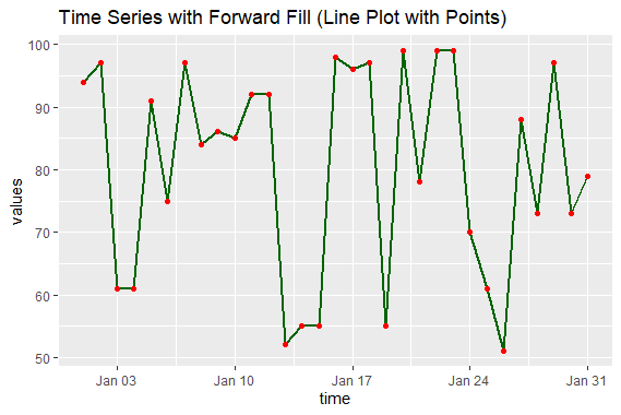
2. Forward Filling

Forward filling involves filling missing values with the most recent observed value,

R

# Forward fill
time_series_data_fill <- na.locf(time_series_data)

# Forward fill with line plot and points
fill_line_point_plot <- ggplot(data.frame(time = index(time_series_data_fill),
                                          values = coredata(time_series_data_fill)),
                               aes(x = time, y = values)) +
  geom_line(color = "darkgreen", size = 1) +
  geom_point(color = "red", size = 1.5) +
  ggtitle("Time Series with Forward Fill (Line Plot with Points)")

fill_line_point_plot

Output:

Time Series with Forward Fill

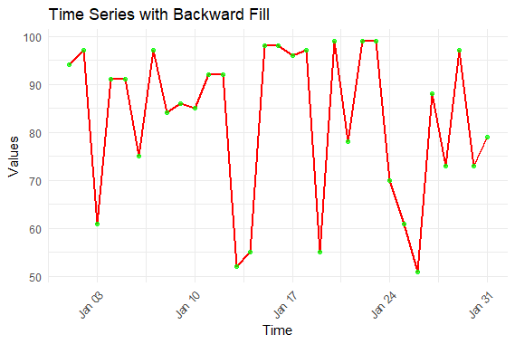
3. Backward Filling

Backward filling involves filling missing values with the next observed value,

R

# Backward fill with na.locf
time_series_data_backfill <- na.locf(time_series_data, fromLast = TRUE)

# Visualize with backward fill in an attractive line plot
backfill_plot <- ggplot(data.frame(time = index(time_series_data_backfill),
                                   values = coredata(time_series_data_backfill)),
                        aes(x = time, y = values)) +
  geom_line(color = "red", size = 1) +  # Adjust line color and size
  geom_point(color = "green", size = 1.5, alpha = 0.7) +
  theme_minimal() +  # Use a minimal theme
  labs(title = "Time Series with Backward Fill",  # Add title
       x = "Time",  # Label for x-axis
       y = "Values") +  # Label for y-axis
  scale_x_date(date_labels = "%b %d", date_breaks = "1 week") +
  theme(axis.text.x = element_text(angle = 45, hjust = 1))

backfill_plot

Output:

Handling Missing Values in Time Series Data

Conclusion

In conclusion, the proper handling of missing values in time series data is a critical aspect of ensuring the reliability and accuracy of analyses. Throughout this article, we explored various techniques to address missing values, each with its own advantages and considerations.