Geospatial Data Analysis with R

Geospatial data analysis involves working with data that has a geographic or spatial component. It allows us to analyze and visualize data in the context of its location on the Earth’s surface. R Programming Language is a popular open-source programming language, that offers a wide range of packages and tools for geospatial data analysis.

fundamental concepts of Geospatial data

1. Spatial Data Types

Vector Data: Geospatial vector data represent discrete geographical features as points, lines, and polygons. Points can be used for locations, lines for linear features like roads, and polygons for areas such as administrative boundaries.

Raster Data: Raster data represents geographic features as a grid of cells, where each cell has a value. This type of data is suitable for continuous or gridded data, such as satellite imagery and elevation data.

2. Coordinate Reference Systems (CRS):

Geospatial data relies on coordinate reference systems to define locations on the Earth’s surface. Common CRS include WGS84 (GPS coordinates) and UTM (Universal Transverse Mercator). You must understand CRS to work with geospatial data effectively.

3. Geospatial Packages:

R offers several packages for geospatial data analysis, including:

1. sf (Simple Features): This package provides a modern, efficient data structure for representing spatial data.
2. rgdal: It offers functions to read and write geospatial data in various formats.
3. sp: This package provides classes and methods for spatial data manipulation and visualization.
4. raster: It is used for working with raster data and performing spatial operations on grids.

Example 1: Importing and Plotting Spatial Data (Vector)

R

# Load the sf package
library(sf)

# Read a shapefile containing polygon data
world <- st_read(system.file("shape/nc.shp", package="sf"))

# Plot the spatial data
plot(world)

Output:

Introduction to Geospatial Data Analysis with R

we load the sf package and read a shapefile containing polygon data representing North Carolina counties. We then plot the spatial data using the plot() function.

Example 2: Raster Data Analysis

R

# Load required packages
library(raster)

# Read a raster dataset (elevation data)
elevation <- raster(system.file("external/test.grd", package="raster"))

# Compute statistics on the elevation data
elev_summary <- summary(elevation)

# Display the summary statistics
print(elev_summary)

Output:

             test
Min.     138.7071
1st Qu.  293.9575
Median   371.9001
3rd Qu.  501.0102
Max.    1736.0580
NA's    6022.0000

In this example, we use the raster package to read a raster dataset containing elevation data. We then compute summary statistics, such as minimum, maximum, and mean elevation, using the summary() function. The result, elev_summary, provides information about the elevation dataset.

Plot the graph for Geospatial Data in R

R

# Install and load necessary packages if you haven't already
install.packages("ggplot2")
install.packages("maps")
install.packages("plotly")

library(ggplot2)
library(maps)
library(plotly)

# Load earthquake data from the 'quakes' dataset
data(quakes)

# Create a basic map of earthquake occurrences
world_map <- map_data("world")
ggplot() +
  geom_polygon(data = world_map, aes(x = long, y = lat, group = group),
               fill = "white", color = "black") +
  geom_point(data = quakes, aes(x = long, y = lat, size = mag,
                                color = depth), alpha = 0.7) +
  scale_size_continuous(range = c(1, 10)) +
  scale_color_gradient(low = "blue", high = "red") +
  labs(
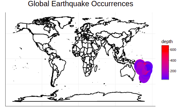
    title = "Global Earthquake Occurrences",
    subtitle = "Magnitude and Depth",
    x = "",
    y = ""
  ) +
  theme_void() +
  theme(plot.title = element_text(hjust = 0.5, size = 18),
        plot.subtitle = element_text(hjust = 0.5, size = 14))

# Make the plot interactive using plotly
earthquake_plot <- ggplotly()

# Display the interactive plot
earthquake_plot

Output:

Introduction to Geospatial Data Analysis with R

• ggplot(): We initialize the plot.
• geom_polygon(): We add a layer for drawing the world map with white fill and black borders.
• geom_point(): We add a layer for plotting earthquake occurrences as points. We map the longitude (long) to the x-axis, latitude (lat) to the y-axis, magnitude (mag) to the size of points, and depth (depth) to the color of points. The alpha parameter controls the transparency of points.
• scale_size_continuous(): We customize the size range of the points.
• scale_color_gradient(): We customize the color scale of the points from blue (low depth) to red (high depth).
• labs(): We set the plot title, subtitle, and axis labels.
• theme_void(): We use a minimal theme with no background.
• theme(plot.title): We further customize the appearance of the plot by adjusting the title’s size and position.

Example 3 using rgdal (Reading and Plotting Spatial Data)

R

# Load the rgdal package
library(rgdal)

# Read a shapefile containing polygon data
world <- readOGR(dsn = system.file("vectors", package = "rgdal"), layer = "world")

# Plot the spatial data
plot(world, col = "lightblue", main = "World Map")

Output:

Introduction to Geospatial Data Analysis with R

In this example, we use the rgdal package to read a shapefile containing polygon data representing countries of the world. We use the readOGR() function to read the shapefile, and then we use the plot() function to visualize the spatial data. We specify the col argument to set the fill color for the polygons and add a title to the plot.

Example 4 using sp (Spatial Data Manipulation and Visualization)

R

# Load the sp package
library(sp)

# Create a simple SpatialPointsDataFrame
coords <- data.frame(
  x = c(0, 1, 2),
  y = c(0, 1, 0)
)
points <- SpatialPoints(coords)
df <- data.frame(ID = c("A", "B", "C"))
spdf <- SpatialPointsDataFrame(points, df)

# Plot the SpatialPointsDataFrame
plot(spdf, pch = 19, col = "red", main = "Simple SpatialPointsDataFrame")

Output:

Introduction to Geospatial Data Analysis with R

In this example, we use the sp package to create a simple SpatialPointsDataFrame. We define coordinates (x and y) for three points, create a data frame for attribute data, and then combine them into a SpatialPointsDataFrame. Finally, we use the plot() function to visualize the points. We specify the pch argument to set the point type, the col argument to set the point color, and add a title to the plot.