Gaussian Mixture Models (GMM) Covariances in Scikit Learn

Gaussian Mixture Models (GMMs) are a type of probabilistic model used for clustering and density estimation. They assist in representing data as a combination of different Gaussian distributions, where each distribution is characterized by its mean, covariance, and weight.

The Gaussian mixture model probability distribution class allows us to estimate the parameters of such a mixture distribution.

In this article, we’ll delve into four types of covariances with GMM models.

GMM in Scikit-Learn

In Scikit-Learn, the GaussianMixture class is used for GMM-based clustering and density estimation. The covariances within GMMs play a vital role in shaping the individual Gaussian components of the mixture.

GaussianMixture includes several parameters such as n_components, covariance_type, tol, reg_covar, max_iter, n_init, init_params, weights_init, means_init, precisions_init, random_state, warm_start, verbose, and verbose_interval. While we won’t discuss all of these in detail within this article to keep it concise, we will explore them in a separate article. For now, let’s focus on understanding the covariance_type parameter more thoroughly.

Understanding and selecting the appropriate covariance type is an important aspect of utilizing GMMs effectively for tasks such as clustering and density estimation. It involves considerations of the inherent structure and relationships within the data.

Covariance Types in Gaussian Mixture

In Gaussian Mixture Models, there are four covariance types available:

1. Full: Each component has its own general covariance matrix, allows each component to have a unique shape, orientation, and size in all dimensions.
2. Tied: All components share the same general covariance matrix, forces all components to share the same shape and orientation, promoting a more spherical distribution.
3. Diag: Each component has its own diagonal covariance matrix, permits components to have different variances along each dimension but assumes no correlation between dimensions.
4. Spherical: Each component has its own single variance, assumes that the shape of each component is spherical, with a single variance for all dimensions

These covariance types in Gaussian Mixture offer flexibility in modeling the distribution of data.

Working with GMM Covariances in Scikit-Learn

To work with GMM covariances in Scikit-Learn, let’s delve deeper into the model with in-built wine dataset.

Step 1: Importing Required Libraires

The very first step is to import the necessary libraries. When working with GMM covariances in Scikit-Learn, it’s essential to have the Scikit-Learn library. An important consideration is to ensure that the library is already installed in your Python environment to avoid any import errors.

Here, we specifically need the “GaussianMixture” module from Scikit-Learn, so we will import Scikit-Learn. Additionally, we will import the NumPy library to facilitate data manipulation. To import these libraries, you can use the following code:

Python3

import numpy as np
import matplotlib.pyplot as plt
from sklearn import datasets
from sklearn.mixture import GaussianMixture
from sklearn.decomposition import PCA

Step 2: Data Preparation

Data preparation is a crucial step in our program. Ensuring that our data is in the correct format for GMM is essential. We must prepare our data accordingly. To begin, let’s load wine dataset for this task, we will leverage the NumPy library.

Python3

# Step 2: Data Preparation
# Load the wine dataset
wine = datasets.load_wine()
X = wine.data[:, :2]

Step 3: Initializing Gaussian Mixture Model:

In this step, we will initialize a Gaussian Mixture Model. To do this, we specify two key parameters:

1. Number of Components: This parameter determines the number of components in our model, and it reflects the number of clusters or distributions the data will be divided into.
2. Covariance Type: The covariance type defines the structure of the covariance matrix for each component. It can be set to one of the four options: full, tied, diag, or spherical.

To work with Gaussian Mixture in Scikit-Learn, we will use the sklearn.mixture module. Within this module, we will set the number of components and the desired covariance type as per our analysis needs.

Python3

n_components = 2  # Number of clusters
covariance_types = ['full', 'tied', 'diag', 'spherical']

Step 4: Fitting the GMM Model:

In this step, we will fit our GMM model using our prepared data. This fitting process will estimate the model’s parameters, including the specified covariance type, along with other essential components. Fitting the GMM model is a crucial step that helps us understand the underlying structure of the data and how it relates to the chosen covariance type.

Python3

# Initialize GMM models for each covariance type
gmm_models = {cov_type: GaussianMixture(n_components=n_components, covariance_type=cov_type)
              for cov_type in covariance_types}

# Step 4: Fitting the GMM Models
# Fit GMM models for each covariance type
for cov_type, gmm_model in gmm_models.items():
    gmm_model.fit(X)

Step 5: Accessing Covariances

You can access the covariance matrices of the components through the “covariances_” attribute of our fitted GMM model. The shape of these covariance matrices depends on the specified ‘covariance_type‘. This will help accessing the covariances.

Python3

covariances = {cov_type: gmm_model.covariances_
               for cov_type, gmm_model in gmm_models.items()}

Step 6: Using the GMM Model for Clustering or Predictions

With our GMM model fully prepared, the final step is to utilize the model for clustering or making predictions, depending on the specific task at hand.

Python3

# Predict the cluster assignments for all data points
predictions = {cov_type: gmm_model.predict(X)
               for cov_type, gmm_model in gmm_models.items()}

Step 7 : Visualizations

Python3

# Plot the clusters for each covariance type
plt.figure(figsize=(12, 8))

for i, (cov_type, gmm_model) in enumerate(gmm_models.items(), 1):
    plt.subplot(2, 2, i)
    plt.scatter(X[:, 0], X[:, 1], c=predictions[cov_type], cmap='viridis', edgecolors='k', s=40)
    plt.title(f'GMM Clustering with {cov_type} Covariance')
    plt.xlabel('Feature 1')
    plt.ylabel('Feature 2')
    plt.colorbar()

    # Print the covariance matrix for the first component (adjust as needed)
    print(f'Covariance Matrix ({cov_type} - Component):\n{covariances[cov_type][0]}')

plt.tight_layout()
plt.show()

Output:

Covariance Matrix (full - Component):
[[0.56109026 0.35297462]
 [0.35297462 1.19112946]]
Covariance Matrix (tied - Component):
[0.65472811 0.06104194]
Covariance Matrix (diag - Component):
[0.77470501 0.13064663]
Covariance Matrix (spherical - Component):
0.5103645862915432

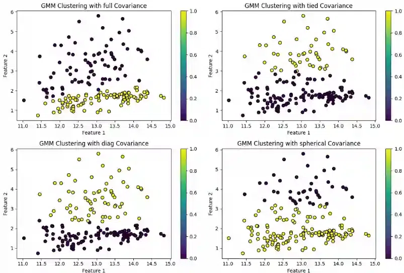
Gaussian Mixture Model

All four plots show the relationship between the number of clusters and the BIC score.

The BIC score is a measure of how well a model fits the data while also penalizing for model complexity. In general, a lower BIC score indicates a better model.

• The plots show that using full covariance generally leads to a better BIC score than using tied, diagonal, or spherical covariance. This means that using full covariance allows the model to better capture the data’s true distribution, even if it comes at the cost of being more complex.
• However, there are some exceptions. For example, in the plot for Feature 2, using tied covariance results in a lower BIC score than using full covariance for a small number of clusters. This suggests that the data in Feature 2 may be well-represented by a simpler model in this case.

Overall, the choice of covariance structure can have a significant impact on the performance of GMM clustering. It is important to experiment with different options to find the one that best fits the data. Choosing an appropriate covariance type is often task-dependent.

For datasets with varying shapes and orientations, ‘full’ covariance might be more suitable. In cases where components are expected to have similar shapes, ‘tied’ or ‘spherical’ covariance might be more appropriate.

Conclusion

Gaussian Mixture Models offer flexible clustering with diverse covariance structures. Model selection, especially covariance type, impacts performance; choose wisely for optimal results.