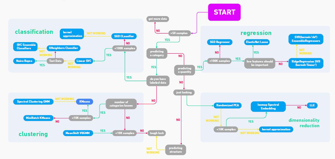
Flowchart for basic Machine Learning models
Last Updated :
05 Sep, 2020
Machine learning tasks have been divided into three categories, depending upon the feedback available:
- Supervised Learning: These are human builds models based on input and output.
- Unsupervised Learning: These are models that depend on human input. No labels are given to the learning algorithm, the model has to figure out the structure by itself.
- Reinforcement learning: These are the models that are feed with human inputs. No labels are given to the learning algorithm. The algorithm learns by the rewards and penalties given.
The algorithms that can be used for each of the categories are:
| Algorithm |
Supervised |
Unsupervised |
Reinforcement |
| Linear |
1 |
0 |
0 |
| Logistic |
1 |
0 |
0 |
| K-Means |
1 |
1 |
0 |
| Anomaly Detection |
1 |
1 |
0 |
| Neural Net |
1 |
1 |
1 |
| KNN |
1 |
0 |
0 |
| Decision Tee |
1 |
0 |
0 |
| Random Forest |
1 |
0 |
0 |
| SVM |
1 |
0 |
0 |
| Naive Bayes |
1 |
0 |
0 |
The machine learning functions and uses for various tasks are given in the below table. To know more about the Algorithms click here.
|
Category
|
Algorithm
|
Function
|
Use
|
| Basic Regression |
Linear |
linear_model.LinearRegression() |
Lots of numerical data |
| Logistic |
linear_model.LogisticRegression() |
Target variable is categorical |
| Cluster Analysis |
K-Means |
cluster.KMeans() |
Similar datum into groups based on centroids |
| Anomaly Detection |
covariance.EllipticalEnvelope() |
Finding outliers through grouping |
| Classification |
Neural Net |
neural_network.MLPClassifier() |
Complex relationships. Prone to over fitting. |
| K-NN |
neighbors.KNeighborsClassifier() |
Group membership based on proximity |
| Decision Tee |
tree.DecisionTreeClassifier() |
If/then/else. Non-contiguous data. Can also be regression. |
| Random Forest |
ensemble.RandomForestClassifier() |
Find best split randomly. Can also be regression |
| SVM |
svm.SVC()
svm.LinearSVC()
|
Maximum margin classifier. Fundamental. Data Science algorithm |
| Naive Bayes |
GaussianNB() MultinominalNB() BernoulliNB() |
Updating knowledge step by step with new info |
| Feature Reduction |
T-DISTRIB Stochastic NEIB Embedding |
manifold.TSNE() |
Visual high dimensional data. Convert similarity to joint probabilities |
| Principle Component Analysis |
decomposition.PCA() |
Distill feature space into components that describe the greatest variance |
| Canonical Correlation Analysis |
decomposition.CCA() |
Making sense of cross-correlation matrices |
| Linear Discriminant Analysis |
lda.LDA() |
Linear combination of features that separates classes |
The flowchart given below will help you give a rough guide of each estimator that will help to know more about the task and the ways to solve it using various ML techniques.
Share your thoughts in the comments
Please Login to comment...