Epsilon-Greedy Algorithm in Reinforcement Learning
Last Updated :
10 Jan, 2023
In Reinforcement Learning, the agent or decision-maker learns what to do—how to map situations to actions—so as to maximize a numerical reward signal. The agent is not explicitly told which actions to take, but instead must discover which action yields the most reward through trial and error.
Multi-Armed Bandit Problem
The multi-armed bandit problem is used in reinforcement learning to formalize the notion of decision-making under uncertainty. In a multi-armed bandit problem, an agent(learner) chooses between k different actions and receives a reward based on the chosen action.
The multi-armed bandits are also used to describe fundamental concepts in reinforcement learning, such as rewards, timesteps, and values.
For selecting an action by an agent, we assume that each action has a separate distribution of rewards and there is at least one action that generates maximum numerical reward. Thus, the probability distribution of the rewards corresponding to each action is different and is unknown to the agent(decision-maker). Hence, the goal of the agent is to identify which action to choose to get the maximum reward after a given set of trials.
Action-Value and Action-Value Estimate
For an agent to decide which action yields the maximum reward, we must define the value of taking each action. We use the concept of probability to define these values using the action-value function.
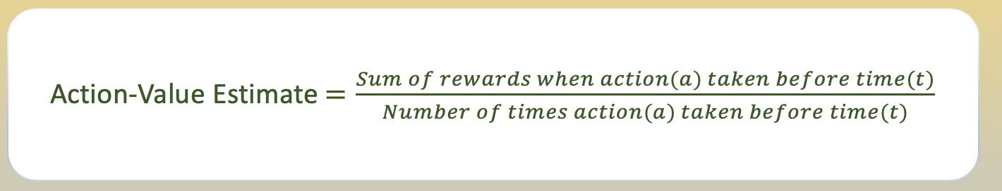
The value of selecting an action is defined as the expected reward received when taking that action from a set of all possible actions. Since the value of selecting an action is not known to the agent, so we use the ‘sample-average’ method to estimate the value of taking an action.
Exploration vs Exploitation
Exploration allows an agent to improve its current knowledge about each action, hopefully leading to long-term benefit. Improving the accuracy of the estimated action-values, enables an agent to make more informed decisions in the future.
Exploitation on the other hand, chooses the greedy action to get the most reward by exploiting the agent’s current action-value estimates. But by being greedy with respect to action-value estimates, may not actually get the most reward and lead to sub-optimal behaviour.
When an agent explores, it gets more accurate estimates of action-values. And when it exploits, it might get more reward. It cannot, however, choose to do both simultaneously, which is also called the exploration-exploitation dilemma.
Epsilon-Greedy Action Selection
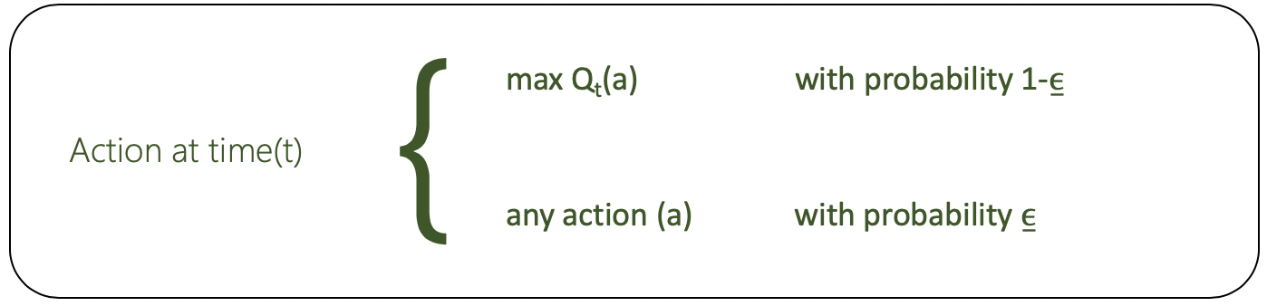
Epsilon-Greedy is a simple method to balance exploration and exploitation by choosing between exploration and exploitation randomly.
The epsilon-greedy, where epsilon refers to the probability of choosing to explore, exploits most of the time with a small chance of exploring.

Code: Python code for Epsilon-Greedy
import numpy as np
import matplotlib.pyplot as plt
class Actions:
def __init__(self, m):
self.m = m
self.mean = 0
self.N = 0
def choose(self):
return np.random.randn() + self.m
def update(self, x):
self.N += 1
self.mean = (1 - 1.0 / self.N)*self.mean + 1.0 / self.N * x
def run_experiment(m1, m2, m3, eps, N):
actions = [Actions(m1), Actions(m2), Actions(m3)]
data = np.empty(N)
for i in range(N):
p = np.random.random()
if p < eps:
j = np.random.choice(3)
else:
j = np.argmax([a.mean for a in actions])
x = actions[j].choose()
actions[j].update(x)
data[i] = x
cumulative_average = np.cumsum(data) / (np.arange(N) + 1)
plt.plot(cumulative_average)
plt.plot(np.ones(N)*m1)
plt.plot(np.ones(N)*m2)
plt.plot(np.ones(N)*m3)
plt.xscale('log')
plt.show()
for a in actions:
print(a.mean)
return cumulative_average
if __name__ == '__main__':
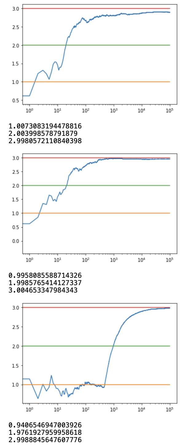
c_1 = run_experiment(1.0, 2.0, 3.0, 0.1, 100000)
c_05 = run_experiment(1.0, 2.0, 3.0, 0.05, 100000)
c_01 = run_experiment(1.0, 2.0, 3.0, 0.01, 100000)
|
Output:
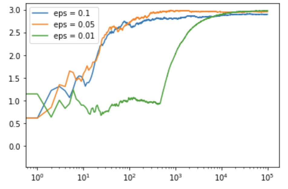
Code: Python code for getting the log output plot
plt.plot(c_1, label ='eps = 0.1')
plt.plot(c_05, label ='eps = 0.05')
plt.plot(c_01, label ='eps = 0.01')
plt.legend()
plt.xscale('log')
plt.show()
|
Output:
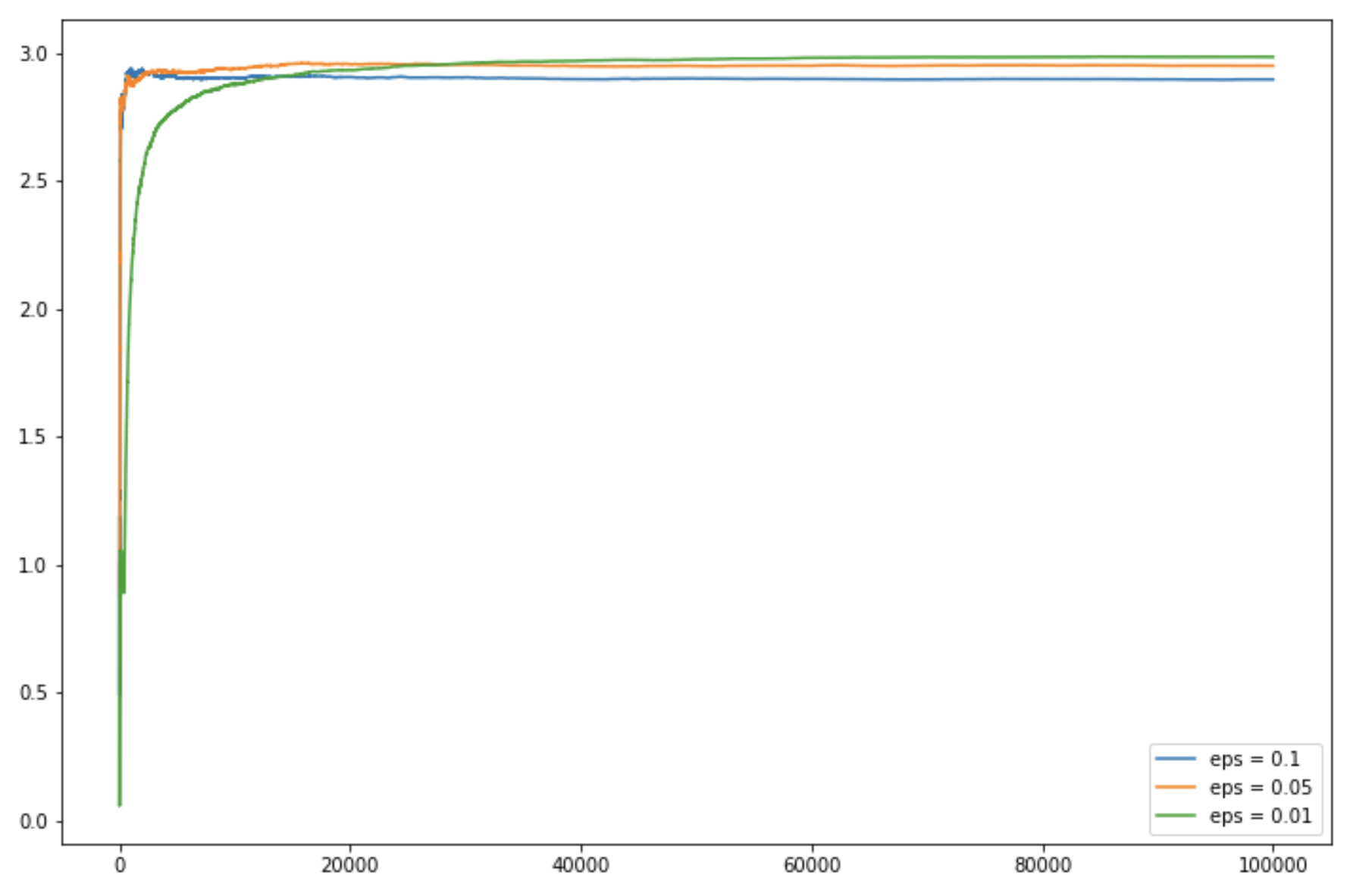
Code: Python code for getting the linear output plot
plt.figure(figsize = (12, 8))
plt.plot(c_1, label ='eps = 0.1')
plt.plot(c_05, label ='eps = 0.05')
plt.plot(c_01, label ='eps = 0.01')
plt.legend()
plt.show()
|
Output:
Share your thoughts in the comments
Please Login to comment...