Compare effect of different scalers on data with outliers in Scikit Learn

Feature scaling is an important step in data preprocessing. Several machine learning algorithms like linear regression, logistic regression, and neural networks rely on the fine-tuning of weights and biases to generalize better. However, features with different scales could prevent such models from performing well as features with higher values dominate the ones with lower values. Scikit Learn offers a variety of scalers to perform feature scaling. This article briefly describes the effect of different scalers on data with outliers.

For demonstration purposes, the California Housing Dataset of Scikit Learn is considered. This dataset consists of 8 attributes and the task is to predict the median house value is $100,000.

Importing required libraries

Python3

# Import the necessary libraries
import numpy as np
import pandas as pd
import matplotlib.pyplot as plt
from sklearn.datasets import fetch_california_housing
from sklearn.model_selection import train_test_split

from sklearn.preprocessing import MinMaxScaler
from sklearn.preprocessing import MaxAbsScaler
from sklearn.preprocessing import StandardScaler
from sklearn.preprocessing import RobustScaler
from sklearn.preprocessing import PowerTransformer
from sklearn.preprocessing import QuantileTransformer
from sklearn.preprocessing import Normalizer
from sklearn.metrics import mean_squared_error
from sklearn.linear_model import SGDRegressor
import seaborn as sns

Load the dataset

Python3

data = fetch_california_housing(as_frame=True)
df = data.frame
df.head()

Output:

	MedInc	HouseAge	AveRooms	AveBedrms	Population	AveOccup	Latitude	Longitude	MedHouseVal
0	8.3252	41.0	6.984127	1.023810	322.0	2.555556	37.88	-122.23	4.526
1	8.3014	21.0	6.238137	0.971880	2401.0	2.109842	37.86	-122.22	3.585
2	7.2574	52.0	8.288136	1.073446	496.0	2.802260	37.85	-122.24	3.521
3	5.6431	52.0	5.817352	1.073059	558.0	2.547945	37.85	-122.25	3.413
4	3.8462	52.0	6.281853	1.081081	565.0	2.181467	37.85	-122.25	3.422

Data information

Python3

df.info()

Output:

<class 'pandas.core.frame.DataFrame'>
RangeIndex: 20640 entries, 0 to 20639
Data columns (total 9 columns):
 #   Column       Non-Null Count  Dtype  
---  ------       --------------  -----  
 0   MedInc       20640 non-null  float64
 1   HouseAge     20640 non-null  float64
 2   AveRooms     20640 non-null  float64
 3   AveBedrms    20640 non-null  float64
 4   Population   20640 non-null  float64
 5   AveOccup     20640 non-null  float64
 6   Latitude     20640 non-null  float64
 7   Longitude    20640 non-null  float64
 8   MedHouseVal  20640 non-null  float64
dtypes: float64(9)
memory usage: 1.4 MB

Now, let us analyze the distribution of each feature.

Python3

# Figure size
plt.figure(figsize=(15,12))
# columns
cols = df.columns

# Distribution plot
for i in range(len(cols)):
    # Subplot
    plt.subplot(3,3,i+1)
    #Distribution plot
    sns.distplot(df[cols[i]], kde = False)

plt.show()

Output:

Distribution plots

We can observe that median income has a long tail distribution, while average occupants have a few large outliers. Hence, we consider these 2 features for studying the impact of different scalers on outliers. Furthermore, let us see the impact of latitude and longitude on the target variable.

Plot Median House value with respect to Latitude and longitude

Python3

lat_long_plot = sns.scatterplot(y = df['Latitude'],
                                x = df['Longitude'],
                                data = df,
                                size = df['MedHouseVal'],
                                hue = df['MedHouseVal'],
                                palette = 'viridis')
lat_long_plot.set_xlabel('Longitude')
lat_long_plot.set_ylabel('Latitude')

Output:

Effect of latitude and longitude on median house value

We can observe that houses from a particular region have high values. Hence, latitude and longitude are also considered for training the model. Ultimately, latitude, longitude, and median income are used to train the model. Now the dataset is split into training and test sets.

Split Train and Test Data

Python3

X_train, X_test, Y_train, Y_test = train_test_split(df,
                                                    df['MedHouseVal'],
                                                    test_size = 0.25,
                                                    random_state=42)

Define the Joint Distribution Plot function

Here we define the function which can plot joint distributions plot for data.

Python3

'''
    # plots the joint plot between median income and average occupants
'''
def plot_dist(data):
    plt.figure(figsize=(8, 5))
    sns.jointplot(x =data[0:1000, 0], y = data[0:1000, 5], data = data)
    plt.show()

Define the Regression model

Here we define the Stochastic Gradient Descent regressor to build the model, then fit the model and predict on X_test new data, then apply mean squared error to find the accuracy of the model.

Python3

def linear_reg(X_train, Y_train, X_test, Y_test):
    reg_model = SGDRegressor()
    reg_model.fit(X_train, Y_train)
    pred = reg_model.predict(X_test)
    accuracy = mean_squared_error(Y_test, pred)
    return accuracy

Without scaling the data

Python3

# Plot the joint distribution for first 1000 datasets
plot_dist(X_train.values)

# without feature scaling
acc = linear_reg(X_train, Y_train, X_test, Y_test)
print(f'MSE  : {acc}')

Output:

Without Scaling the data

MSE  : 1.3528478529652859e+29

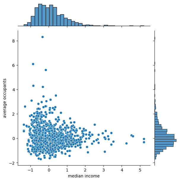
Effect of Standard Scaler

Scikit Learn offers StandardScaler() for performing standardization.

Python3

# performing standardization
std_scaler = StandardScaler()

X_train_std_scaler = std_scaler.fit_transform(X_train)
X_test_std_scaler  = std_scaler.transform(X_test)

# Plot the joint distribution
plot_dist(X_train_std_scaler)

# with standard scaler
acc = linear_reg(X_train_std_scaler, Y_train, X_test_std_scaler, Y_test)
print(f'Accuracy with standard scaler : {acc}')

Output:

Effect of Standard Scaler

Accuracy with standard scaler : 2.927062092029926e-07

We can observe that the scales of the 2 features are quite different. The median income is ranging from -2 to 6, whereas the average occupants is ranging from -0.1 to 0.6. Therefore, standard scalers cannot guarantee balanced feature scales.

Effect of MinMax Scaler

Scikit Learn offers MinMaxScaler() for normalization.

Python3

# performing min_max_scaler
min_max_scaler = MinMaxScaler()

X_train_min_max_scaler = min_max_scaler.fit_transform(X_train)
X_test_min_max_scaler = min_max_scaler.transform(X_test)

# Plot the joint distribution
plot_dist(X_train_min_max_scaler)

# with minmax scaler
acc = linear_reg(X_train_min_max_scaler, Y_train, X_test_min_max_scaler, Y_test)
print(f'Accuracy with minmax scaler : {acc}')

Output:

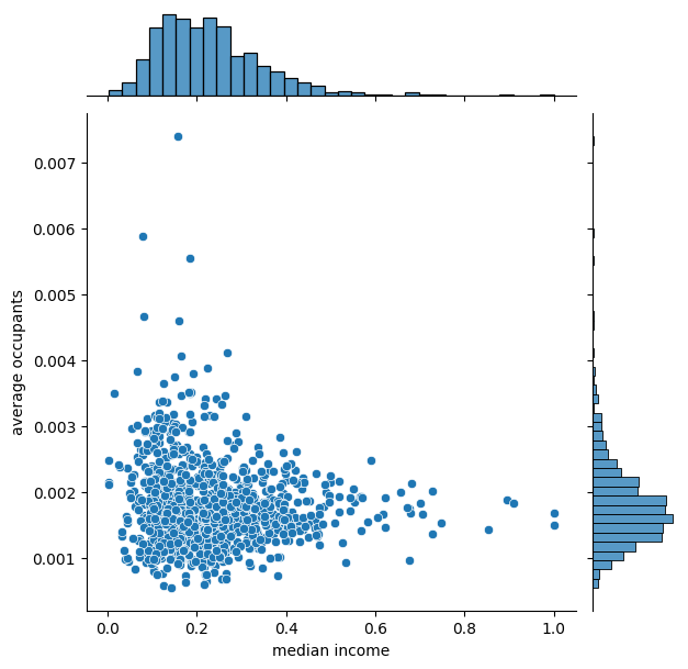
Effect of MinMax Scaler

Accuracy with minmax scaler : 0.005800840622553663

MinMax scaler reduces the range of feature values to [0, 1]. However, the range is quite different for the 2 features under consideration. Average occupants have a considerably smaller value compared to median income.

Effect of MaxAbs Scaler

MaxAbsScaler() is similar to MinMaxScaler(). However, the range of scaled values may vary depending on the feature values. The range is [0, 1] if only positive values are present, [-1, 0] if only negative values are present, and [-1, 1] if both values are present.

Python3

max_abs_scaler = MaxAbsScaler()

X_train_max_abs_scaler = max_abs_scaler.fit_transform(X_train)
X_test_max_abs_scaler = max_abs_scaler.transform(X_test)

# Plot the joint distribution
plot_dist(X_train_max_abs_scaler)

# with maxabs scaler
acc = linear_reg(X_train_max_abs_scaler, Y_train, X_test_max_abs_scaler, Y_test)
print(f'Accuracy with maxabs scaler : {acc}')

Output:

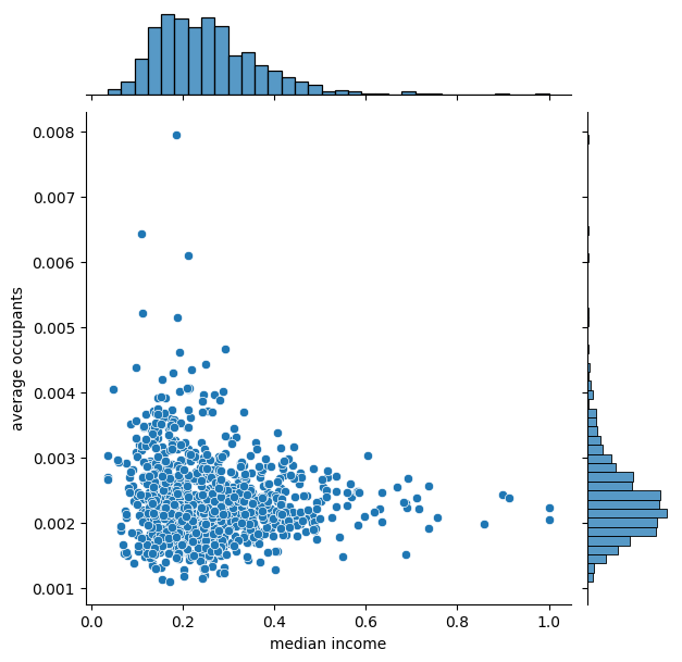
Effect of Max Absolute Scaler

Accuracy with maxabs scaler : 0.006259459937552328

In this case, it produces results similar to MinMaxScaler().

Effect of Robust Scaler

Scikit Learn provides RobustScaler() which makes use of inter-quartile range for feature scaling.

Python3

robust_scaler = RobustScaler()

X_train_robust_scaler = robust_scaler.fit_transform(X_train)
X_test_robust_scaler = robust_scaler.transform(X_test)

# Plot the joint distribution
plot_dist(X_train_robust_scaler)

# with robust scaler
acc = linear_reg(X_train_robust_scaler, Y_train, X_test_robust_scaler, Y_test)
print(f'Accuracy with robust scaler : {acc}')

Output:

Effect of Robust Scaler

Accuracy with robust scaler : 1.931800745764342e+20

Effect of Power Transform

Python3

power_transform = PowerTransformer()

X_train_power_transform = power_transform.fit_transform(X_train)
X_test_power_transform = power_transform.transform(X_test)

# Plot the joint distribution
plot_dist(X_train_power_transform)

# with power transform
acc = linear_reg(X_train_power_transform, Y_train, X_test_power_transform, Y_test)
print(f'Accuracy with power transform    : {acc}')

Output:

Effect of Power Transform

Accuracy with power transform    : 0.09313345304679063

Effect of Quantile Transformer

Python3

quantiles = QuantileTransformer(n_quantiles=23, random_state=0)

X_train_quantiles = quantiles.fit_transform(X_train)
X_test_quantiles = quantiles.transform(X_test)

# Plot the joint distribution
plot_dist(X_train_quantiles)

# with QuantileTransformer
acc = linear_reg(X_train_quantiles, Y_train, X_test_quantiles, Y_test)
print(f'Accuracy with QuantileTransformer: {acc}')

Output:

Effect of Quantile Transformer

Effect of Normalizer

Python3

from sklearn.preprocessing import Normalizer

normalize = Normalizer()

X_train_normalize = normalize.fit_transform(X_train)
X_test_normalize = normalize.transform(X_test)

# Plot the joint distribution
plot_dist(X_train_normalize)

# with Normalizer
acc = linear_reg(X_train_normalize, Y_train, X_test_normalize, Y_test)
print(f'Accuracy with Normalizer : {acc}')

Output:

Effect of Normalizer

Accuracy with Normalizer : 1.3216531944583318

Model Accuracy

Let’s print the accuracy of each model

Python3

# without feature scaling
acc = linear_reg(X_train, Y_train, X_test, Y_test)
print(f'General Accuracy                 : {acc}')

# with standard scaler
acc = linear_reg(X_train_std_scaler, Y_train, X_test_std_scaler, Y_test)
print(f'Accuracy with standard scaler    : {acc}')

# with minmax scaler
acc = linear_reg(X_train_min_max_scaler, Y_train, X_test_min_max_scaler, Y_test)
print(f'Accuracy with minmax scaler      : {acc}')

# with maxabs scaler
acc = linear_reg(X_train_max_abs_scaler, Y_train, X_test_max_abs_scaler, Y_test)
print(f'Accuracy with maxabs scaler      : {acc}')

# with robust scaler
acc = linear_reg(X_train_robust_scaler, Y_train, X_test_robust_scaler, Y_test)
print(f'Accuracy with robust scaler      : {acc}')

# with power transform
acc = linear_reg(X_train_power_transform, Y_train, X_test_power_transform, Y_test)
print(f'Accuracy with power transform    : {acc}')

# with QuantileTransformer
acc = linear_reg(X_train_quantiles, Y_train, X_test_quantiles, Y_test)
print(f'Accuracy with QuantileTransformer: {acc}')

# with Normalizer
acc = linear_reg(X_train_normalize, Y_train, X_test_normalize, Y_test)
print(f'Accuracy with Normalizer         : {acc}')

Output:

General Accuracy                 : 2.6731951662759754e+28
Accuracy with standard scaler    : 6.1103137019148144e-06
Accuracy with minmax scaler      : 0.005842587280784744
Accuracy with maxabs scaler      : 0.006149996463712555
Accuracy with robust scaler      : 1.0374102250716266e+23
Accuracy with power transform    : 0.09243653923790224
Accuracy with QuantileTransformer: 0.12639279065095635
Accuracy with Normalizer         : 1.322663822919674

It is evident that feature scaling improves accuracy significantly. In the current scenario, feature scaling with standard scaler and min-max scaler provides the best accuracy.