Agglomerative clustering with different metrics in Scikit Learn

Agglomerative clustering is a type of Hierarchical clustering that works in a bottom-up fashion. Metrics play a key role in determining the performance of clustering algorithms. Choosing the right metric helps the clustering algorithm to perform better. This article discusses agglomerative clustering with different metrics in Scikit Learn.

Scikit learn provides various metrics for agglomerative clusterings like Euclidean, L1, L2, Manhattan, Cosine, and Precomputed. Let us take a look at each of these metrics in detail:

• Euclidean Distance: It measures the straight line distance between 2 points in space.
• Manhattan Distance: It measures the sum of absolute differences between 2 points/vectors in all dimensions.
• Cosine Similarity: It measures the angular cosine similarity between 2 vectors.

Agglomerative Clustering

Two kinds of datasets are considered, low dimensional and high dimensional. High-dimensional data has more features than data records. For low-dimensional data, the customer shopping dataset is considered. This dataset has 5 features namely, Customer Id, Gender, Age, Annual Income (k$), and Spending Score (1-100). We will form clusters based on Annual Income (k$) and Spending Score (1-100) as scatter plots between other features do not show promising patterns. For high dimensional data, the forest cover type dataset is considered that has 55 features and 5,81,012 data records. However, to convert this dataset into a high-dimensional dataset only 50 records are considered for clustering.

Python3

import numpy as np
import pandas as pd
import matplotlib.pyplot as plt
from sklearn import preprocessing
import scipy.cluster.hierarchy as sch
from sklearn.cluster import AgglomerativeClustering
from sklearn.metrics import silhouette_score

Load the datasets using the panda’s data frame.

Python3

# low dimensional data
df = pd.read_csv("Mall_Customers.csv")

# high dimensional data
hd_df = pd.read_csv("covtype.csv")
hd_data = hd_df.head(50)

Let’s take a look at the first five rows of the low-dimensional dataset.

Python3

df.head()

Output:

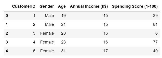
First five rows of the dataset

Function for implementing agglomerative clustering using different metrics.

Python3

# generates clusters using agglomerative clustering algorithm
# uses average linkage method with different affinity (metric) values

def agg_clustering(data, num_clusters, metric):
    cluster_model = AgglomerativeClustering(n_clusters=num_clusters,
                                            affinity=metric,
                                            linkage='average')

    clusters = cluster_model.fit_predict(data)

    score = silhouette_score(data,
                             cluster_model.labels_,
                             metric='euclidean')
    return clusters, score

Scaling the data and invoking the above function.

Python3

X = df.iloc[:, [3, 4]].values

scaler = preprocessing.StandardScaler()
scaled_X = scaler.fit_transform(X)

y_euclidean, euclidean_score = agg_clustering(scaled_X, 5, 'euclidean')
y_l1, l1_score = agg_clustering(scaled_X, 5, 'l1')
y_l2, l2_score = agg_clustering(scaled_X, 5, 'l2')
y_manhattan, manhattan_score = agg_clustering(scaled_X, 5, 'manhattan')
y_cosine, cosine_score = agg_clustering(scaled_X, 5, 'cosine')

Let’s plot the clusters. 

Python3

# plots the clusters formed using different metrics
# y contains cluster labels for each data record

def plot_clusters(data, y, metric):
    plt.scatter(data[y==0, 0], data[y==0, 1],
                s=100, c='red',
                label ='Cluster 1')
    plt.scatter(data[y==1, 0], data[y==1, 1],
                s=100, c='blue',
                label ='Cluster 2')
    plt.scatter(data[y==2, 0], data[y==2, 1],
                s=100, c='green',
                label ='Cluster 3')
    plt.scatter(data[y==3, 0], data[y==3, 1],
                s=100, c='purple',
                label ='Cluster 4')
    plt.scatter(data[y==4, 0], data[y==4, 1],
                s=100, c='orange',
                label ='Cluster 5')

    plt.title(f'Clusters of Customers (using {metric} distance metric)')
    plt.xlabel('Annual Income(k$)')
    plt.ylabel('Spending Score(1-100)')
    plt.legend()
    plt.show()

Python3

plot_clusters(X, y_euclidean, 'euclidean')
plot_clusters(X, y_l1, 'l1')
plot_clusters(X, y_l2, 'l2')
plot_clusters(X, y_manhattan, 'manhattan')
plot_clusters(X, y_cosine, 'cosine')

Output:

It is a bit difficult to figure out the differences between the clusters formed using different metrics just by looking at the above plots. Hence, we make use of silhouette scores to compare the above clusters.

Python3

silhouette_scores = {'euclidean': euclidean_score,
                     'l1': l1_score,
                     'l2': l2_score,
                     'manhattan': manhattan_score,
                     'cosine': cosine_score}
plt.bar(list(silhouette_scores.keys()),
        list(silhouette_scores.values()),
        width=0.4)

Output:

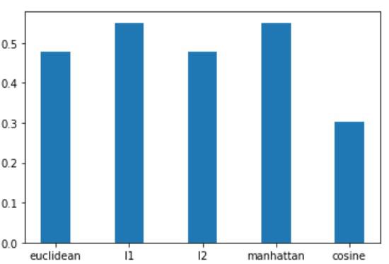
Comparison of different metrics for clusters formed

We can observe that Manhattan or L1 metric and Euclidean or L2 metric give good silhouette scores. However, the cosine metric performs poorly in this case. Cosine metric gives a poor performance with low dimensional data and should be avoided. Also, data must be scaled before using Euclidean or L2 distance metric.

Similarly, clusters are formed for high dimensional data after scaling the features.

Python3

numerical_features = ["Elevation", "Aspect", "Slope",
                      "Horizontal_Distance_To_Hydrology",
                      "Vertical_Distance_To_Hydrology",
                      "Horizontal_Distance_To_Roadways",
                      "Hillshade_9am", "Hillshade_Noon",
                      "Hillshade_3pm",
                      "Horizontal_Distance_To_Fire_Points"]
hd_data[numerical_features] = scaler.fit_transform(hd_data[numerical_features])

y_hd_euclidean, euclidean_score_hd = agg_clustering(hd_data, 5, 'euclidean')
y_hd_l1, l1_score_hd = agg_clustering(hd_data, 5, 'l1')
y_hd_l2, l2_score_hd = agg_clustering(hd_data, 5, 'l2')
y_hd_manhattan, manhattan_score_hd = agg_clustering(hd_data, 5, 'manhattan')
y_hd_cosine, cosine_score_hd = agg_clustering(hd_data, 5, 'cosine')

Let’s take a look at the silhouette scores.

Python3

silhouette_scores_hd = {'euclidean': euclidean_score_hd,
                        'l1': l1_score_hd,
                        'l2': l2_score_hd,
                        'manhattan': manhattan_score_hd,
                        'cosine': cosine_score_hd}
plt.bar(list(silhouette_scores_hd.keys()),
        list(silhouette_scores_hd.values()),
        width=0.4)

Output:

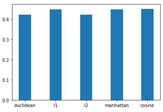
Comparison of different metrics for clusters formed

In this case, the cosine metric performs pretty well. Hence, cosine is generally used with high-dimensional data. Manhattan or L1 metric also performs well on high dimensional data. However, the Euclidean metric does not perform very well on high-dimensional data due to the “curse of dimensionality”.