Build a simple Quantum Circuit using IBM Qiskit in Python

Qiskit is an open source framework for quantum computing. It provides tools for creating and manipulating quantum programs and running them on prototype quantum devices on IBM Q Experience or on simulators on a local computer. Let’s see how we can create simple Quantum circuit and test it on a real Quantum computer or simulate in our computer locally. Python is a must prerequisite for understanding Quantum programs as Qiskit itself is developed using Python.

First and foremost part before entering into the subject is installation of Qiskit and Anaconda. Refer to the below articles for step by step guide for anaconda installation.

• How to install Anaconda on windows?
• How to install Anaconda on Linux?

Installation

To install qiskit follow the below steps:

• Open Anaconda Prompt and type

pip install qiskit

• That’s it, this will install all necessary packages.
• Next, open Jupyter Notebook.
• Import qiskit using the following command.

import qiskit

To get access to IBM Quantum Systems:

1. Create a free IBM Quantum Experience Account.
2. Navigate to My Account.
3. Click on Copy Token to copy the token to the clipboard(Token represents the API to access IBM Quantum devices).
4. Run the following commands(Jupyter Notebook) to store your API token locally for later use in a configuration file called qiskitrc. Replace MY_API_TOKEN with the API token.

from qiskit import IBMQ
IBMQ.save_account('MY_API_TOKEN')

Getting Started

Firstly, we will import the necessary packages. The import lines import the basic elements (packages and functions) needed for your program.                              

The imports used in the code example are:

• QuantumCircuit: Holds all your quantum operations; the instructions for the quantum system
• execute: Runs your circuit
• Aer: Handles simulator backends
• qiskit.visualization: Enables data visualization, such as plot_histogram

Initialize variables

In the next line of code, you initialize two qubits in the zero state, and two classical bits in the zero state, in the quantum circuit called circuit.

Add gates

The next three lines of code, beginning with circuit., add gates that manipulate the qubits in your circuit.

Detailed Explanation

• QuantumCircuit.h(0): A Hadamard gate on qubit 0, which puts it into a superposition state
• QuantumCircuit.cx(0, 1): A controlled-NOT operation (C_x ) on control qubit 0 and target qubit 1, putting the qubits in an entangled state
• QuantumCircuit.measure([0,1], [0,1]): The first argument indexes the qubits, the second argument indexes the classical bits. The nth qubit’s measurement result will be stored in the nth classical bit.

This particular trio of gates added one-by-one to the circuit forms the Bell state,|

In this state, there is a 50 percent chance of finding both qubits to have the value zero and a 50 percent chance of finding both qubits to have the value one.

Simulate the experiment

The next line of code calls a specific simulator framework – in this case, it calls Qiskit Aer, which is a high-performance simulator that provides several backends to achieve different simulation goals. In this program, we will use the qasm_simulator. Each run of this circuit will yield either the bit string ’00’ or ’11’. The program specifies the number of times to run the circuit in the shots argument of the execute method (job = execute(circuit, simulator, shots=1000)). The number of shots of the simulation is set to 1000 (the default is 1024). Once you have a result object, you can access the counts via the method get_counts(circuit). This gives you the aggregate outcomes of your experiment. The output bit string is ’00’ approximately 50 percent of the time. This simulator does not model noise. Any deviation from 50 percent is due to the small sample size.

Visualize the circuit

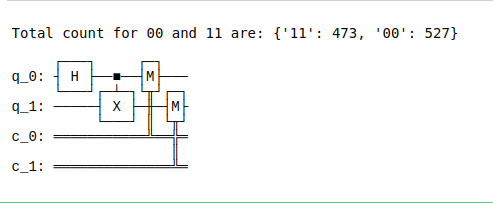
QuantumCircuit.draw() (called by circuit.draw() in the code) displays your circuit in one of the various styles used in textbooks and research articles. In the circuit obtained after visualization command , the qubits are ordered with qubit zero at the top and qubit one below it. The circuit is read from left to right, representing the passage of time.

Visualize the results

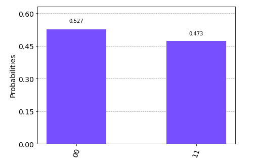
Qiskit provides many visualizations, including the function plot_histogram, to view your results.

plot_histogram(counts)

The probabilities (relative frequencies) of observing the |00? and |11? states are computed by taking the respective counts and dividing by the total number of shots.

Below is the implementation.

Python3

# python program to create a simple Quantum circuit


%matplotlib inline
from qiskit import QuantumCircuit, execute, Aer, IBMQ
from qiskit.compiler import transpile, assemble
from qiskit.tools.jupyter import *
from qiskit.visualization import *

# Loading your IBM Q account(s)
provider = IBMQ.load_account()

# Create a Quantum Circuit acting
# on the q register
circuit = QuantumCircuit(2, 2)

# Add a H gate on qubit 0
circuit.h(0)

# Add a CX (CNOT) gate on control
# qubit 0 and target qubit 1
circuit.cx(0, 1)

# Map the quantum measurement to the
# classical bits
circuit.measure([0,1], [0,1])

# Use Aer's qasm_simulator
simulator = Aer.get_backend('qasm_simulator')

# Execute the circuit on the qasm
# simulator
job = execute(circuit, simulator, shots=1000)

# Grab results from the job
result = job.result()

# Return counts
counts = result.get_counts(circuit)
print("\nTotal count for 00 and 11 are:",counts)

# Draw the circuit
circuit.draw()

Output:

Plot a histogram

Python3

# Plot a histogram
plot_histogram(counts)

Output: