Audio Recognition in Tensorflow

This article discusses audio recognition and also covers an implementation of a simple audio recognizer in Python using the TensorFlow library which recognizes eight different words.

Audio Recognition

Audio recognition comes under the automatic speech recognition (ASR) task which works on understanding and converting raw audio to human-understandable text. It is popularly known as speech-to-text (STT) and this technology is widely used in our day-to-day applications. Some of the popular examples include meeting transcriptions in Zoom meetings, virtual speech assistants like Alexa, and voice searches in Google search.

The main goal behind ASR is to accurately convert speech to text while taking into consideration any background noise, a person’s speaking style, accent, and any other factor. Once speech has been accurately transcribed into text, this information can be further processed and used for a wide range of tasks, such as identifying user commands in virtual speech assistants or providing text-based search results in voice search applications.

Implementation

Now, to process the audio signals, we would first convert them to spectrograms, which are basically 2D image representations of change in frequency over time. Later we will use these spectrogram images to train a model to identify the words based on patterns in spectrogram signals. The following subsections contain more details about the dataset, model architecture, training method, and testing of the trained model.

Step 1: Importing Libraries, Dataset, and Preprocessing

In this article, we would be using the following libraries.

Python3

import os
import tensorflow as tf
import numpy as np
import seaborn as sns
import pathlib
from IPython import display
from matplotlib import pyplot as plt
from sklearn.metrics import classification_report

Step 2: Download the dataset

Now, for implementing a simple audio recognizer we would be using mini speech commands dataset by Google which contains audio of eight different words spoken by different people. The words in the dataset include “yes”, “no”, “up”, “down”, “left”, “right”, “on”, and “off”. To download the dataset use the following code:

Python3

# Downloading the mini_speech_commands dataset from the external URL
data = tf.keras.utils.get_file(
  'mini_speech_commands.zip',
  origin="http://storage.googleapis.com/download.tensorflow.org/data/mini_speech_commands.zip",
  extract=True,
  cache_dir='.', cache_subdir='data')

Check the directory

Python3

os.listdir('./data/')

Output:

['mini_speech_commands.zip', '__MACOSX', 'mini_speech_commands']

Step 3: Preprocessing

Split the data into the Training and validation set

Splitting the data into training and validation sets and getting the labels.

Python3

# Using audio_dataset_from_directory function to create dataset with audio data
training_set, validation_set = tf.keras.utils.audio_dataset_from_directory(
    directory='./data/mini_speech_commands',
    batch_size=16,
    validation_split=0.2,
    output_sequence_length=16000,
    seed=0,
    subset='both')

# Extracting audio labels
label_names = np.array(training_set.class_names)
print("label names:", label_names)

Output:

Found 8000 files belonging to 8 classes.
Using 6400 files for training.
Using 1600 files for validation.
label names: ['down' 'go' 'left' 'no' 'right' 'stop' 'up' 'yes']

Drop the extra axis in the audio channel data

Now, we will applying tf.squeeze function to drop the extra axis in the audio channel data.

Python3

# Defining the squeeze function
def squeeze(audio, labels):
  audio = tf.squeeze(audio, axis=-1)
  return audio, labels

# Applying the function on the dataset obtained from previous step
training_set = training_set.map(squeeze, tf.data.AUTOTUNE)
validation_set = validation_set.map(squeeze, tf.data.AUTOTUNE)

Waveform

Visualize a sample waveform from the processed dataset.

Python3

# Visualize the waveform
audio, label = next(iter(training_set))
display.display(display.Audio(audio[0], rate=16000))

Output:

Listen it

Spectrogram

Now, we will convert the audio to a spectrogram and visualize it.

Python3

# Plot the waveform
def plot_wave(waveform, label):
    plt.figure(figsize=(10, 3))
    plt.title(label)
    plt.plot(waveform)
    plt.xlim([0, 16000])
    plt.ylim([-1, 1])
    plt.xlabel('Time')
    plt.ylabel('Amplitude')
    plt.grid(True)

# Convert waveform to spectrogram
def get_spectrogram(waveform):
    spectrogram = tf.signal.stft(waveform, frame_length=255, frame_step=128)
    spectrogram = tf.abs(spectrogram)
    return spectrogram[..., tf.newaxis]

# Plot the spectrogram
def plot_spectrogram(spectrogram, label):
    spectrogram = np.squeeze(spectrogram, axis=-1)
    log_spec = np.log(spectrogram.T + np.finfo(float).eps)
    plt.figure(figsize=(10, 3))
    plt.title(label)
    plt.imshow(log_spec, aspect='auto', origin='lower')
    plt.colorbar(format='%+2.0f dB')
    plt.xlabel('Time')
    plt.ylabel('Frequency')

# Plotting the waveform and the spectrogram of a random sample
audio, label = next(iter(training_set))

# Plot the wave with its label name
plot_wave(audio[0], label_names[label[0]])

# Plot the spectrogram with its label name
plot_spectrogram(get_spectrogram(audio[0]), label_names[label[0]])

Output:

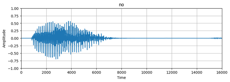
Plot of audio wave

Audio spectrogram

Create input dataset and split Validation set into two parts

Now, creating a spectrogram dataset from the audio dataset and also splitting the validation set into two parts, one for validation during training and another for testing the trained model.

Python3

# Creating spectrogram dataset from waveform or audio data
def get_spectrogram_dataset(dataset):
    dataset = dataset.map(
        lambda x, y: (get_spectrogram(x), y),
        num_parallel_calls=tf.data.AUTOTUNE)
    return dataset

# Applying the function on the audio dataset
train_set = get_spectrogram_dataset(training_set)
validation_set = get_spectrogram_dataset(validation_set)

# Dividing validation set into two equal val and test set
val_set = validation_set.take(validation_set.cardinality() // 2)
test_set = validation_set.skip(validation_set.cardinality() // 2)

Check the dimension of the input dataset

Python3

train_set_shape = train_set.element_spec[0].shape
val_set_shape = val_set.element_spec[0].shape
test_set_shape = test_set.element_spec[0].shape

print("Train set shape:", train_set_shape)
print("Validation set shape:", val_set_shape)
print("Testing set shape:", test_set_shape)

Output:

Train set shape: (None, 124, 129, 1)
Validation set shape: (None, 124, 129, 1)
Testing set shape: (None, 124, 129, 1)

Step 4: Build the model

Now, since we have converted our audio data to image format, this problem has turned into a classification problem and we can define a simple CNN model to train and classify these audio.

Python3

# Defining the model
def get_model(input_shape, num_labels):
    model = tf.keras.Sequential([
        tf.keras.layers.Input(shape=input_shape),
        # Resizing the input to a square image of size 64 x 64 and normalizing it
        tf.keras.layers.Resizing(64, 64),
        tf.keras.layers.Normalization(),

        # Convolution layers followed by MaxPooling layer
        tf.keras.layers.Conv2D(64, 3, activation='relu'),
        tf.keras.layers.Conv2D(128, 3, activation='relu'),
        tf.keras.layers.MaxPooling2D(),
        tf.keras.layers.Dropout(0.5),
        tf.keras.layers.Flatten(),

        # Dense layer
        tf.keras.layers.Dense(256, activation='relu'),
        tf.keras.layers.Dropout(0.5),

        # Softmax layer to get the label prediction
        tf.keras.layers.Dense(num_labels, activation='softmax')
    ])
    # Printing model summary
    model.summary()
    return model

# Getting input shape from the sample audio and number of classes
input_shape = next(iter(train_set))[0][0].shape
print("Input shape:", input_shape)
num_labels = len(label_names)

# Creating a model
model = get_model(input_shape, num_labels)

Output:

Input shape: (124, 129, 1)
Model: "sequential_1"
_________________________________________________________________
 Layer (type)                Output Shape              Param #   
=================================================================
 resizing_1 (Resizing)       (None, 64, 64, 1)         0         
                                                                 
 normalization_1 (Normalizat (None, 64, 64, 1)         3         
 ion)                                                            
                                                                 
 conv2d_2 (Conv2D)           (None, 62, 62, 64)        640       
                                                                 
 conv2d_3 (Conv2D)           (None, 60, 60, 128)       73856     
                                                                 
 max_pooling2d_1 (MaxPooling (None, 30, 30, 128)       0         
 2D)                                                             
                                                                 
 dropout_2 (Dropout)         (None, 30, 30, 128)       0         
                                                                 
 flatten_1 (Flatten)         (None, 115200)            0         
                                                                 
 dense_2 (Dense)             (None, 256)               29491456  
                                                                 
 dropout_3 (Dropout)         (None, 256)               0         
                                                                 
 dense_3 (Dense)             (None, 8)                 2056      
                                                                 
=================================================================
Total params: 29,568,011
Trainable params: 29,568,008
Non-trainable params: 3
_________________________________________________________________

Step 5: Model Training and Validation

Now, we will compile and train the model. Since this is a multiclass classification problem, we will be using categorical cross entropy as loss function to improve the model.

Python3

model.compile(
    optimizer=tf.keras.optimizers.Adam(),
    loss=tf.keras.losses.SparseCategoricalCrossentropy(),
    metrics=['accuracy'],
)

EPOCHS = 10
history = model.fit(
    train_set,
    validation_data=val_set,
    epochs=EPOCHS,
)

Output:

Epoch 1/10
400/400 [==============================] - 241s 600ms/step - loss: 1.4206 - accuracy: 0.5186 - val_loss: 0.7907 - val_accuracy: 0.7900
Epoch 2/10
400/400 [==============================] - 284s 711ms/step - loss: 0.7536 - accuracy: 0.7570 - val_loss: 0.6210 - val_accuracy: 0.7950
Epoch 3/10
400/400 [==============================] - 305s 762ms/step - loss: 0.5214 - accuracy: 0.8273 - val_loss: 0.4603 - val_accuracy: 0.8600
Epoch 4/10
400/400 [==============================] - 341s 853ms/step - loss: 0.4128 - accuracy: 0.8594 - val_loss: 0.4495 - val_accuracy: 0.8562
Epoch 5/10
400/400 [==============================] - 340s 849ms/step - loss: 0.3295 - accuracy: 0.8908 - val_loss: 0.4215 - val_accuracy: 0.8600
Epoch 6/10
400/400 [==============================] - 337s 844ms/step - loss: 0.2721 - accuracy: 0.9086 - val_loss: 0.4133 - val_accuracy: 0.8725
Epoch 7/10
400/400 [==============================] - 331s 829ms/step - loss: 0.2499 - accuracy: 0.9192 - val_loss: 0.4623 - val_accuracy: 0.8662
Epoch 8/10
400/400 [==============================] - 338s 845ms/step - loss: 0.2092 - accuracy: 0.9283 - val_loss: 0.4528 - val_accuracy: 0.8737
Epoch 9/10
400/400 [==============================] - 339s 847ms/step - loss: 0.2018 - accuracy: 0.9316 - val_loss: 0.3762 - val_accuracy: 0.8938
Epoch 10/10
400/400 [==============================] - 339s 848ms/step - loss: 0.1811 - accuracy: 0.9397 - val_loss: 0.4379 - val_accuracy: 0.8662

Plotting validation and training loss and accuracy.

Python3

# Plotting the history
metrics = history.history
plt.figure(figsize=(10, 5))

# Plotting training and validation loss
plt.subplot(1, 2, 1)
plt.plot(history.epoch, metrics['loss'], metrics['val_loss'])
plt.legend(['loss', 'val_loss'])
plt.xlabel('Epoch')
plt.ylabel('Loss')

# Plotting training and validation accuracy
plt.subplot(1, 2, 2)
plt.plot(history.epoch, metrics['accuracy'], metrics['val_accuracy'])
plt.legend(['accuracy', 'val_accuracy'])
plt.xlabel('Epoch')
plt.ylabel('Accuracy')

Output:

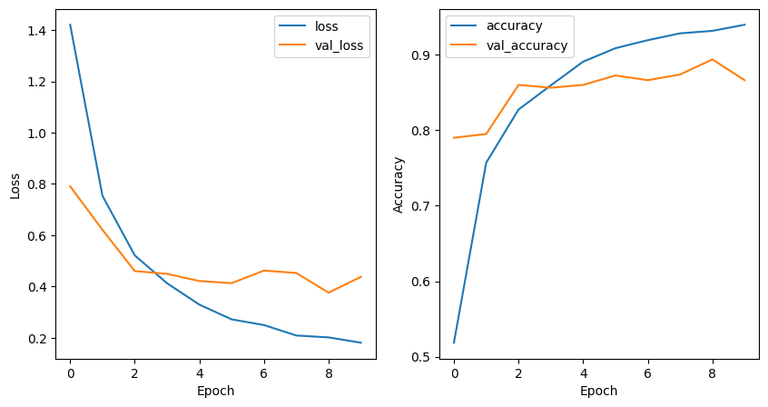
Validation Vs Training loss and accuracy

Step 6: Model Evaluation

For evaluation we will use a confusion matrix to see how well the model performed on the testing set.

Python3

# Confusion matrix
y_pred = np.argmax(model.predict(test_set), axis=1)
y_true = np.concatenate([y for x, y in test_set], axis=0)
cm = tf.math.confusion_matrix(y_true, y_pred)

# Plotting the confusion matrix
plt.figure(figsize=(10, 8))
sns.heatmap(cm, annot=True, fmt='g')
plt.xlabel('Predicted')
plt.ylabel('Actual')
plt.show()

Output:

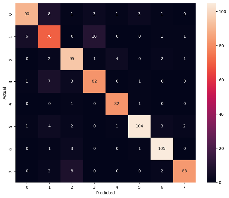
Confusion Matrix

Classification Report

Python3

report = classification_report(y_true, y_pred)
print(report)

Output:

              precision    recall  f1-score   support

           0       0.85      0.85      0.85       107
           1       0.70      0.78      0.74        88
           2       0.90      0.90      0.90       105
           3       0.84      0.85      0.85        94
           4       0.94      0.95      0.95        84
           5       0.96      0.86      0.91       117
           6       0.86      0.91      0.88       110
           7       0.97      0.89      0.93        95

    accuracy                           0.88       800
   macro avg       0.88      0.88      0.88       800
weighted avg       0.88      0.88      0.88       800

Step :7  Audio Recognization

Python3

path = 'data/mini_speech_commands/yes/004ae714_nohash_0.wav'
Input = tf.io.read_file(str(path))
x, sample_rate = tf.audio.decode_wav(Input, desired_channels=1, desired_samples=16000,)
audio, labels = squeeze(x, 'yes')

waveform = audio
display.display(display.Audio(waveform, rate=16000))

x = get_spectrogram(audio)
x = tf.expand_dims(x, axis=0)

prediction = model(x)
plt.bar(label_names, tf.nn.softmax(prediction[0]))
plt.title('Prediction : '+label_names[np.argmax(prediction, axis=1).item()])
plt.show()

Output:

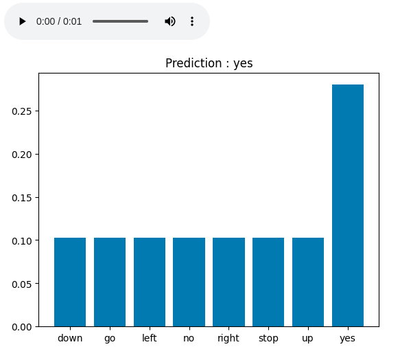
Audio Recognization Result