Age and Gender Prediction using CNN

In this article, we will create an Age and Gender Prediction model using Keras Functional API, which will perform both Regression to predict the Age of the person and Classification to predict the Gender from face of the person.

Age and Gender Prediction

Keras Functional API offers a more flexible and creative way to make models of higher complexity. One such Complexity arises when making a model that does more than one type of supervised prediction (Regression and Classification predictions). We will unravel a similar scenario to create a model that can perform Regression and Classification as well.

Dataset

We will use the Age, Gender (Face Data) CSV dataset for our purpose and to achieve this we will use a Convolutional Neural Network (CNN). CNN is a powerful tool in Deep Learning that helps the user classify an Image and has the most usage in Computer Vision. It enables the Machine to visualize and interpret Images and Image data. For an in-depth explanation of CNN and its architecture.

Prerequisite

The essential libraries we have used are:

• Pandas – An open-source library to read and manipulate datasets. Here it was used to read the CSV file which contained pixel values for the image
• Numpy – An open-source library with functions for high-level mathematical calculations as well as handling data that spans multiple dimensions
• Matlplotlib– An open source library which is used to visualize our data and losses in our prediction model
• Sklearn – This library consists of pre-defined functions and evaluation metrics that help in data preprocessing, model performance evaluation and model initialization.
• Tensorflow – Developed by Google, this open-source library is used for creating Deep learning models. It provides many methods to interpret data but mainly focuses on training and inference of Neural Networks

Importing main libraries

Python3

# importing necessary libraries
import matplotlib.pyplot as plt
import tensorflow as tf
import random
import keras
from keras import layers
from sklearn.model_selection import train_test_split
from tensorflow.keras.callbacks import EarlyStopping

Reading the Dataset

The dataset used here was in a csv format. We used Pandas to read the csv file and print the shape and information about the dataset.

Python3

# reading the dataset
df= pd.read_csv('age_gender.csv')
print(df.head())

Output:

   age  ethnicity  gender                        img_name  \
0    1          2       0  20161219203650636.jpg.chip.jpg   
1    1          2       0  20161219222752047.jpg.chip.jpg   
2    1          2       0  20161219222832191.jpg.chip.jpg   
3    1          2       0  20161220144911423.jpg.chip.jpg   
4    1          2       0  20161220144914327.jpg.chip.jpg   

                                              pixels  
0  129 128 128 126 127 130 133 135 139 142 145 14...  
1  164 74 111 168 169 171 175 182 184 188 193 199...  
2  67 70 71 70 69 67 70 79 90 103 116 132 145 155...  
3  193 197 198 200 199 200 202 203 204 205 208 21...  
4  202 205 209 210 209 209 210 211 212 214 218 21...  

Check the data basic informations

Python3

# information about the dataset
df.info()

Output:

<class 'pandas.core.frame.DataFrame'>
RangeIndex: 23705 entries, 0 to 23704
Data columns (total 5 columns):
 #   Column     Non-Null Count  Dtype 
---  ------     --------------  ----- 
 0   age        23705 non-null  int64 
 1   ethnicity  23705 non-null  int64 
 2   gender     23705 non-null  int64 
 3   img_name   23705 non-null  object
 4   pixels     23705 non-null  object
dtypes: int64(3), object(2)
memory usage: 926.1+ KB

Data Preprocessing

We are concerned about the pixels column in the dataframe. But the values in that column are an object type data type. To convert the datatype of the column, we will define a function which adheres to our purpose at hand and then apply it to create a new column.

Python3

# creating a fuctio which will change the datatype to an array
def str_to_array(ob):
    return np.array(ob.split(' '), dtype='int')

# apply the function to pixels column and create a new column 'new_pixels'
df['new_pixels'] = df['pixels'].apply(str_to_array)

Check the input Face images

To visualize an Image, we are first generating a list of random indices value from the dataset and using that to plot a subplot of images. To plot the image we have to first reshape the data into a (48,48,1) shape.

Python3

# creating an empty 3x3 subplot
fig, ax = plt.subplots(3, 5, figsize=(12, 7))
ax = ax.ravel()

# generating a random list of integers
res = random.sample(range(0, df.shape[0]), 15)

# creating the subplot for random images and printing the corresponding gender and age
for i, id in enumerate(res):
    ax[i].imshow(df['new_pixels'].loc[id].reshape(48, 48))
    ax[i].set_title(f'Age:{df.age.loc[id]}, Gender:{df.gender.loc[id]}')
    ax[i].axis('off')
plt.savefig('image_visualization_subplot.png')

Output:

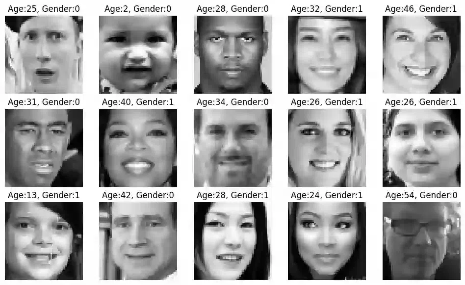
Age and Gender

Model Building

To start with creating the model, we first expand the new pixels column to make a dataframe. Using that dataframe and necessary target values (age and gender), we will split our dataset into training and Validation Dataset.

Python3

# create the X (predictor) variables
X_new = pd.DataFrame(df['new_pixels'].tolist())

# Assign Predictor Variables and Target variables
X = X_new
y_age = df['age'].values
y_gender = df['gender'].values

# split the Variables into Train and Validation sets
y_reg_train, y_reg_val, y_clf_train, y_clf_val, X_train, X_val = train_test_split(y_age,
                                                                                  y_gender,
                                                                                  X,
                                                                                  test_size=0.2,
                                                                                  stratify = y_gender,
                                                                                  random_state=42)
# Check the shape
y_reg_train.shape, y_reg_val.shape, y_clf_train.shape, y_clf_val.shape, X_train.shape, X_val.shape

Output:

((18964,), (4741,), (18964,), (4741,), (18964, 2304), (4741, 2304))

Normalizations

Before we proceed forward, a necessary step in Data preparation for training is to normalize the pixel data. This ensures that the pixels are in a similar data distribution which will help in faster model convergence in training.

Python3

# normalising the Pixel data for training dataset and then reshaping it to (48,48,1)
Xmin = 0
Xmax = 255
X_train = X_train.values
X_train = X_train - Xmin/(Xmax-Xmin)
X_train = X_train.reshape(-1,48,48,1)

# similar step is taken for Validation set
X_val = X_val.values
X_val = X_val - Xmin/(Xmax-Xmin)
X_val = X_val.reshape(-1,48,48,1)

Creating The CNN model Architecture

The model architecture is made using functional API of keras. This method is helpful in joining two types of output (in this case regression and classification) as a single output to be fed to the model.

The Model takes 3 parts:

1. Input: This layer takes in the input data with shape (48,48,1)
2. Middle architecture: All the Deep Learning Networks are cascaded over Input layer, i.e., the input layer is joined with subsequent layers in the deep learning model. In this case the architecture consists of:
   • a single Conv2D layer with 16 node
   • a single Conv2D layer with 32 nodes followed by Maxpooling2D layer
   • two conv2D layer with 64 nodes each
   • a flatten layer
   • two dense layer of 128 and 32 nodes respectively
3. Output: The output of the model consist of two dense layers which corresponds to the necessary task they will perform which are:
   • a dense layer with 1 node and sigmoid activation which will perform the gender classification
   • a dense layer with 1 node and linear activation which will perform the age regression prediction

For all the other layers, necessary activations were provided. To understand the underlying layers and the parameters involved in the model architecture created above, we will plot the model

Python3

input_layer = keras.Input(shape=(48, 48, 1), name="Input image")
x = layers.Conv2D(16, 3, activation="relu")(input_layer)
x = layers.Conv2D(32, 3, activation="relu")(x)
x = layers.MaxPooling2D(3)(x)
x = layers.Conv2D(64, 3, activation="relu")(x)
x = layers.Conv2D(64, 3, activation="relu")(x)
x = layers.Flatten()(x)
x = layers.Dense(128, activation='relu')(x)
x = layers.Dense(32, activation='relu')(x)



out_a = keras.layers.Dense(1, activation='sigmoid', name='g_clf')(x)
out_b = keras.layers.Dense(1, activation='linear', name='a_reg')(x)

model = keras.Model( inputs = input_layer, outputs = [out_a, out_b], name="age_gender_model")

Output:

Model Training

We compile the model with necessary loss, metrics and optimizers (remember to do so for each layer as you will see in the code below) and fitted the model for 200 epochs with an earlystopping of patience 25.

Python3

# compile the model
model.compile(
    loss = {
        "g_clf": 'binary_crossentropy',
        "a_reg": 'mse'
    },

    metrics = {
        "g_clf": 'accuracy',
        "a_reg": 'mse'
    },

    optimizer = tf.keras.optimizers.Adam(learning_rate=0.003)
)

# create an EarlyStopping instance which will stop if the val_loss doesn't change much in 25 epochs
callback = EarlyStopping(monitor='val_loss',
                         patience=25,
                         verbose=0)

# train the model
history = model.fit(X_train,
                    [y_clf_train, y_reg_train],
                    batch_size = 256,
                    validation_data= (X_val, [y_clf_val, y_reg_val]),
                    epochs=200, callbacks = [callback])

Output:

Epoch 1/200
75/75 [==============================] - 79s 662ms/step - loss: 2402.7998 - g_clf_loss: 2.7341 - a_reg_loss: 2400.0664 - g_clf_accuracy: 0.4776 - a_reg_mse: 2400.0664 - val_loss: 423.1724 - val_g_clf_loss: 1.0336 - val_a_reg_loss: 422.1387 - val_g_clf_accuracy: 0.4200 - val_a_reg_mse: 422.1387
Epoch 2/200
75/75 [==============================] - 52s 693ms/step - loss: 357.2810 - g_clf_loss: 1.4903 - a_reg_loss: 355.7906 - g_clf_accuracy: 0.4606 - a_reg_mse: 355.7906 - val_loss: 449.3816 - val_g_clf_loss: 1.4558 - val_a_reg_loss: 447.9258 - val_g_clf_accuracy: 0.5916 - val_a_reg_mse: 447.9258
Epoch 3/200
75/75 [==============================] - 51s 683ms/step - loss: 290.7226 - g_clf_loss: 0.9503 - a_reg_loss: 289.7724 - g_clf_accuracy: 0.6046 - a_reg_mse: 289.7724 - val_loss: 231.5632 - val_g_clf_loss: 0.6586 - val_a_reg_loss: 230.9046 - val_g_clf_accuracy: 0.6748 - val_a_reg_mse: 230.9046
Epoch 4/200
...
Epoch 58/200
75/75 [==============================] - 49s 653ms/step - loss: 19.4069 - g_clf_loss: 0.3974 - a_reg_loss: 19.0095 - g_clf_accuracy: 0.8104 - a_reg_mse: 19.0095 - val_loss: 114.9000 - val_g_clf_loss: 0.4197 - val_a_reg_loss: 114.4803 - val_g_clf_accuracy: 0.8019 - val_a_reg_mse: 114.4803

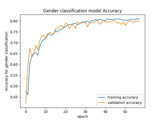
Plotting the Losses and Accuracy for Regression and Classification Respectively

To visualize the losses, we will use history of our model training and plot the necessary metrices.

Python3

# plotting for Gender Classification Accuracy
plt.plot(history.history['g_clf_accuracy'], label = 'training accuracy')
plt.plot(history.history['val_g_clf_accuracy'], label = 'validation accuracy')
plt.title('Gender classification model Accuracy')
plt.xlabel('epoch')
plt.ylabel('Accuracy for gender classification')
plt.legend()
plt.show()

Output:

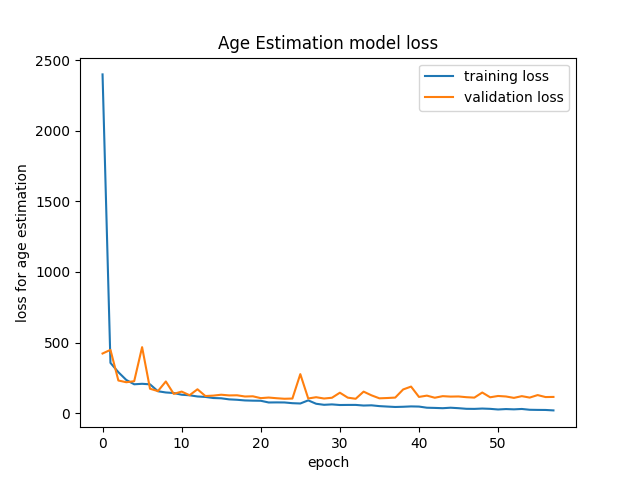
Python3

# plotting the mse loss for age regression
plt.plot(history.history['a_reg_mse'], label = 'training loss')
plt.plot(history.history['val_a_reg_mse'], label = 'validation loss')
plt.title('Age Estimation model loss')
plt.xlabel('epoch')
plt.ylabel('loss for age estimation')
plt.legend()

plt.show()

Output:

Model Evaluations

Python3

model.evaluate(X_val, [y_clf_val, y_reg_val])

Output:

149/149 [==============================] - 3s 18ms/step - loss: 114.9000 - g_clf_loss: 0.4197 - a_reg_loss: 114.4803 - g_clf_accuracy: 0.8019 - a_reg_mse: 114.4803

[114.89997100830078,
 0.4196634590625763,
 114.48027801513672,
 0.8019405007362366,
 114.48027801513672]

Predictn Age & Gender from the model

We created a subplot of 3×3 with random indices and predicted the age and gender for the given input image

Python3

fig, ax = plt.subplots(3,3, figsize = (10,15))

ax = ax.ravel()

res = random.sample(range(0, X_val.shape[0]), 9)

for i,id in enumerate(res):
    ax[i].imshow(X_val[id])
    ax[i].set_title(f'Age-group: {y_reg_val[id]}, Gender: {gender_dict[str(y_clf_val[id])]}')

    pred_Gender, pred_age = model.predict(tf.expand_dims(X_val[id], 0), verbose = 0)
    y_value = np.where(pred_Gender > 0.5, 1,0)
    ax[i].set_xlabel(f'gender: {gender_dict[str(y_value[0][0])]} , age: {int(np.round(pred_age,0))}')

plt.savefig('prediction_subplot.png')

Output:

In the above subplot, the title at the top signifies actual age and gender whereas the title below signifies predicted age and gender. As you can see the predictions are quite good.

Conclusion

We saw how we processed a csv dataframe with object type pixel entries, used then with Functional Keras API and created a Model complex enough that it could Classify the Gender and Predict their Age.