Word2Vec Using R

Word2Vec is a modeling technique used to create word embeddings. It creates a vector of words where it assigns a number to each of the words. Word embeddings generally predict the context of the sentence and predict the next word that can occur. In R Programming Language Word2Vec provides two methods to predict it:

• CBOW (Continuous Bag of Words)
• Skip Gram

The basic idea of word embedding is words that occur in similar contexts tend to be closer to each other in vector space. The vectors are used as input to do specific NLP tasks. The other tasks are text summarization, text matching, etc.

Continuous Bag of Words

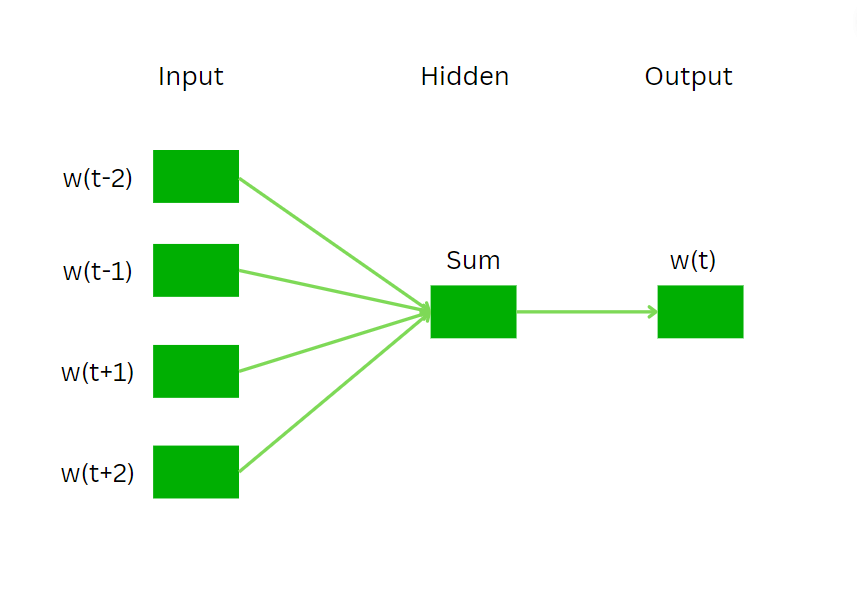
The continuous Bag of Words (CBOW) model aims to predict the target word based on the context provided by the surrounding words. The working of the CBOW is as follows:

1. Step 1: Take the context of surrounding words as input. This is the window of words around the word.
2. Step 2: Each word is represented as a vector in the embedding layer in the given context. The dimensions of the vector stores the information on the semantic and syntactic features of the word.
3. Step 3: Aggregate the individual word ( or vectors) to get a single vector that represents the context. It will become our input.
4. Step 4: Finally predict the output using the input in the previous step. We get a probability distribution over the vocabulary and the word with the highest probability is considered the target word.

CBOW is adjusted using the neural network to minimize the difference between the predicted word and the actual word in the target.

CBOW

• Sentence given: “GeeksforGeeks is a nice website”
• Window size: 2 (within the window of 2 around the target word “nice”)
• Let we want to predict word: nice, so considering 1 word on both sides of the target word, we have
• Input: The context words are “a”, and “website”.
• Each word is represented through a vector of embedding. Then the embeddings are aggregated to create a single vector of context (e.g., by averaging) to create a single vector representing the context.
• Using the aggregated context vector to predict the target word, The model outputs a probability distribution over the vocabulary.

Ouput: The output should predict the word “nice”.

CBOW is trained to efficiently predict target words based on their surrounding context. The neural network learns to represent words in a way that captures their semantic and syntactic relationships, optimizing the overall predictive performance.

Skip Gram

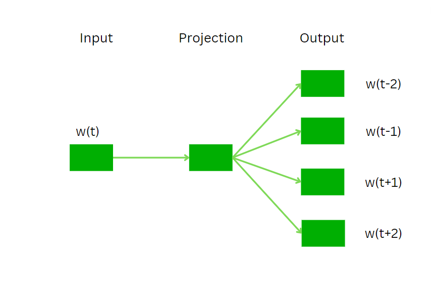
Skip-Gram predicts the context words based on the given target word, contrary to CBOW which predicts the target word. It learns the relationships between words by training the model maximizing the probability of predicting context words given a target word. The working of Skip gram is as follows:

• Step 1: Provide the input word.
• Step 2: Create an embedding layer for the target word by creating a vector.
• Step 3: Using the embedding layer it creates a probability distribution of words over the vocabulary. Then the context words are sampled according to the distribution.

Skip-gram is trained by adjusting the weights of the neural network to maximize the likelihood of predicting the correct context words from the embedding layer.

• Sentence given: “GeeksforGeeks is a nice website”
• Window size: 2 (considering words within a window of 2 around the target word)
• Target word: “nice”.
• Input: “nice”.

For the chosen target word (“nice”), an embedding layer is created representing the word as a vector in a high-dimensional space. The dimensions of this vector are determined by the chosen embedding size during the model training.

• Then using the embedding layer to create a probability distribution over the entire vocabulary based on the target word “nice” and creating sample context words from the probability distribution.
• In this example, let’s say the sampled context words are “a” and “website.”
• Then using the probability distribution, words “a” and “website” is predicted.

The Skip-Gram model is trained to adjust its weights during the training process so that the probability distribution generated from the embedding layer is more likely to predict the correct context words for the given target word.

Continuous Bag of Words for lookalike words

In this example, we load the word2vec library which allows to train a model for word 2 vector and use cbow and skip gram algorithms. We can train model, see embeddings and see nearest words to any word.

Dataset drive link: BRAirlines Dataset

Step 1: Import the libraries word2vec for training the cbow model and data.table for dataframe.

R

# Required Libraries install
install.packages(c("word2vec", "data.table", "tm", "stringr", "ggplot2", "ggrepel",
                   "plotly", "umap"))


# Load the libraries
library(data.table)
library(word2vec)

Step 2: Import the dataset. We will be using Airline reviews as our dataset provided in kaggle.

R

# load dataset
# reference: https://www.kaggle.com/datasets/chaudharyanshul/airline-reviews
data = read.csv("BA_AirlineReviews.csv")
reviews = data$ReviewBody

Step 3: Create the cbow model with the reviews and provide dimension of 15 and maximum iterations 20.

R

# using cbow algorithm
cbow_model = word2vec(x = reviews, type = "cbow", dim = 15, iter = 20)

Step 4: Find the similar context words that are nearest in meaning by using the predict() method and provide the type as nearest.

R

# finding lookalike
cbow_lookslike <- predict(cbow_model, c("hotel", "airbus"), type = "nearest", top_n = 5)
print("The nearest words for hotel and airbus in CBOW model prediction is as follows ")
print(cbow_lookslike)

Output:

[1] "The nearest words for hotel and airbus in CBOW model prediction is as follows "
$hotel
  term1       term2 similarity rank
1 hotel        taxi  0.9038663    1
2 hotel destination  0.8645503    2
3 hotel         bag  0.8606780    3
4 hotel        neck  0.8571329    4
5 hotel     clothes  0.8561315    5
$airbus
   term1      term2 similarity rank
1 airbus     ordeal  0.8780979    1
2 airbus    equally  0.8745981    2
3 airbus uneventful  0.8690495    3
4 airbus        BAH  0.8677440    4
5 airbus      beers  0.8504817    5

Step 5: Find the embeddings of some words as follows by using the predict() method and provide the type as embedding.

R

# checking embeddings
cbow_embedding <- as.matrix(cbow_model)
cbow_embedding <- predict(cbow_model, c("airbus", "plane"), type = "embedding")
print("The CBOW embedding for airbus and plane is as follows ")
print(cbow_embedding)

Output:

[1] "The CBOW embedding for airbus and plane is as follows "
             [,1]       [,2]       [,3]       [,4]      [,5]       [,6]
airbus  0.1426127  0.2532609 -0.6377366 0.02548989 1.6425037 -0.3880948
plane  -0.6500510 -0.4534873  1.1207893 0.50630522 0.3934476 -1.0468076
             [,7]       [,8]       [,9]    [,10]       [,11]      [,12]
airbus  1.4523754 1.51974189 -0.1617979 2.170428 0.147469506  0.1358749
plane  -0.2956116 0.07400164  1.0075779 1.670310 0.004237913 -0.5283979
            [,13]      [,14]     [,15]
airbus -0.2461894 -0.6237084 -1.419138
plane  -1.3195559 -0.8242296 -2.238492

Visualizing the Embeddings in the CBOW Model

Here we will visualize the word embeddings and how the words correlate with each other.

Step 1: Create a corpus of the reviews.

R

# Load necessary libraries
library(tm)
library(stringr)


# Create a corpus
corpus <- Corpus(VectorSource(reviews))

Step 2: Apply some preprocessing for the text to extract the list of words and split them.

R

corpus <- tm_map(corpus, content_transformer(tolower))
corpus <- tm_map(corpus, removePunctuation)
corpus <- tm_map(corpus, removeNumbers)
corpus <- tm_map(corpus, removeWords, stopwords("en"))
corpus <- tm_map(corpus, stripWhitespace)

Step 3: Now we convert it to Document Term Matrix. Next we split the words and extract them.

R

# Create a document-term matrix
dtm <- DocumentTermMatrix(corpus)

# Get the words
words <- colnames(as.matrix(dtm))

# Create a list of words
word_list <- strsplit(words, " ")
word_list <- unlist(word_list)

# Remove empty strings
word_list <- word_list[word_list != ""]

Step 4: We take a list of 100 words from it.

R

word_list = head(word_list, 100)

Step 5: Get the embeddings for the words and drop which dont have embeddings using the na.omit() method. We use the predict() method with type embedding to get the embeddings. It stores the words with there embeddings.

R

# checking embeddings
cbow_embedding <- as.matrix(cbow_model)
cbow_embedding <- predict(cbow_model, word_list, type = "embedding")
cbow_embedding <- na.omit(cbow_embedding)

Step 6: Since the embeddings are high dimensional array, we first scale down it and then plot it using plotly for interactive plotting. For lowering the dimension we use the umap() method from umap library. We provide n_neighbors for how many neighbours to consider as the reduced dimension for this task.

R

library(ggplot2)
library(ggrepel)
library(plotly)
library(umap)
vizualization <- umap(cbow_embedding, n_neighbors = 15, n_threads = 2)

df  <- data.frame(word = rownames(cbow_embedding),
                  xpos = gsub(".+//", "", rownames(cbow_embedding)),
                  x = vizualization$layout[, 1], y = vizualization$layout[, 2],
                  stringsAsFactors = FALSE)

plot_ly(df, x = ~x, y = ~y, type = "scatter", mode = 'text', text = ~word) %>%
  layout(title = "CBOW Embeddings Visualization")

Output:

Skip Gram Embeddings and lookalike words

Step 1: Import the libraries word2vec for training the skip-gram model and data.table for dataframe.

R

# Required Libraries install
install.packages(c("word2vec", "data.table", "tm", "stringr", "ggplot2", "ggrepel", "plotly", "umap"))

# Load the libraries
library(data.table)
library(word2vec)

Step 2: Import the dataset. We will be using Airline reviews as our dataset provided in kaggle.

R

# load dataset
# reference: https://www.kaggle.com/datasets/chaudharyanshul/airline-reviews
data = read.csv("https://gist.githubusercontent.com/ManavSarkar/
33f322600f2cd5a99d90e1cbaa9e8997/raw/a00623af6aba53ce75d7820ef6082587ba0fdc6a/
BA_AirlineReviews.csv")
reviews = data$ReviewBody

Step 3: Create the skip-gram model with the reviews and provide dimension of 15 and maximum iterations 20.

R

# using skip gram algorithm
skip_gram_model = word2vec(x = reviews, type = "skip-gram", dim = 15, iter = 20)

Step 4: Create embeddings using the predict() method provided by word2vec model. Then print the embeddings of any word.

R

# checking embeddings
skip_embedding <- as.matrix(skip_gram_model)
skip_embedding <- predict(skip_gram_model, c("airbus", "plane"), type = "embedding")
print("The SKIP Gram embedding for airbus and plane is as follows ")
print(skip_embedding)

Output:

[1] "The SKIP Gram embedding for airbus and plane is as follows "
             [,1]        [,2]       [,3]      [,4]      [,5]      [,6]
airbus -0.2280359 -0.06950876 -0.8975230 0.2383098 0.9572678 1.3951594
plane  -0.8150198 -0.25508881 -0.2011317 0.6494479 1.1521208 0.6378013
            [,7]      [,8]       [,9]     [,10]     [,11]    [,12]     [,13]
airbus 0.1191502 -1.828172 -0.1717374 0.4359438 0.1890430 2.530286 -1.072369
plane  0.3009279 -1.175530 -0.9957678 0.9003520 0.2462102 1.611048 -1.707145
            [,14]    [,15]
airbus  0.1053236 0.207101
plane  -1.1464180 1.383812

Step 5: Find the similar context words that are nearest in meaning by using the predict() method and provide the type as nearest.

R

# finding lookalike
skip_lookslike <- predict(skip_gram_model, c("hotel", "airbus"), type = "nearest",
                          top_n = 5)
print("The nearest words for hotel and airbus in skip gram model
prediction is as follows ")
print(skip_lookslike)

Output:

[1] "The nearest words for hotel and airbus in skip gram model \nprediction is as follows "
$hotel
  term1          term2 similarity rank
1 hotel  accommodation  0.9651411    1
2 hotel    destination  0.9277243    2
3 hotel            cab  0.9195876    3
4 hotel           taxi  0.9188855    4
5 hotel transportation  0.9100887    5
$airbus
   term1    term2 similarity rank
1 airbus airplane  0.9217460    1
2 airbus   slight  0.9211015    2
3 airbus   itself  0.9184811    3
4 airbus   parked  0.8968953    4
5 airbus     Trip  0.8923244    5

Step 6: Create new embeddings for the words_list. And then draw the visualization.

R

# checking embeddings
skip_embedding <- as.matrix(skip_gram_model)
skip_embedding <- predict(skip_gram_model, word_list, type = "embedding")
skip_embedding <- na.omit(skip_embedding)

library(ggplot2)
library(ggrepel)
library(plotly)
library(umap)
vizualization <- umap(skip_embedding, n_neighbors = 15, n_threads = 2)

df  <- data.frame(word = rownames(skip_embedding),
                  xpos = gsub(".+//", "", rownames(skip_embedding)),
                  x = vizualization$layout[, 1], y = vizualization$layout[, 2],
                  stringsAsFactors = FALSE)

plot_ly(df, x = ~x, y = ~y, type = "scatter", mode = 'text', text = ~word) %>%
  layout(title = "Skig Gram Embeddings Visualization")

Output:

Word2Vec Using R

Conclusion

In conclusion, Word2Vec, employing CBOW and Skip-Gram models, generates powerful word embeddings by capturing semantic relationships. CBOW predicts a target word from its context, while Skip-Gram predicts context words from a target word. These embeddings enable NLP tasks and, as demonstrated with airline reviews, showcase the models’ ability to find contextually similar words.