Weighted Lasso Regression in R

In the world of data analysis and prediction, regression techniques are essential for understanding relationships between variables and making accurate forecasts. One standout method among many is Lasso regression. It not only helps in finding these relationships but also aids in creating models that are easier to interpret and more resilient. However in R Programming Language dealing with imbalanced data or when some data points are more crucial than others, traditional Lasso regression might fall short. That’s where Weighted Lasso Regression steps in. It offers a more sophisticated way of modeling by assigning different levels of importance to various data points.

What is Lasso Regression?

Lasso regression adds a penalty term to ordinary least squares, shrinking less important feature coefficients to zero for variable selection. It aids in building simpler models and mitigating multicollinearity, balancing model simplicity with predictive accuracy. Popular in predictive modeling, it’s effective with large feature sets.

What is Weighted Lasso Regression?

Weighted Lasso regression is a variation of the Lasso regression model that incorporates weights on the predictor variables. In traditional Lasso regression, the penalty term in the objective function is the L1-norm of the coefficients multiplied by a regularization parameter lambda. This penalty encourages sparsity in the coefficient estimates, effectively shrinking some coefficients towards zero and setting others to exactly zero.

In Weighted Lasso regression, each predictor variable is assigned a weight, and these weights are used to scale the penalty term. The purpose of assigning weights is to prioritize or emphasize certain predictors over others based on their importance or relevance in the regression model. Variables with higher weights contribute more to the penalty term, thereby influencing the coefficient estimates more strongly.

[Tex]\min_{\beta} \left\{ \frac{1}{2n} \sum_{i=1}^{n} w_i (y_i – x_i^T\beta)^2 + \lambda \sum_{j=1}^{p} |\beta_j| \right\} [/Tex]

• n: Number of observations.
• p: Number of predictors.
• wi: Weights assigned to each observation.
• λ: Lasso regularization parameter.
• yi: Observed response for the i-th observation.
• xi: Vector of predictors for the i-th observation.
• β: Coefficient vector to be estimated.

The first term in the objective function represents the least squares loss function, which measures the discrepancy between the observed response and the predicted response based on the current coefficient estimates. The second term represents the penalty term, which is the L1-norm of the coefficient vector multiplied by the weights. This term encourages sparsity in the coefficient estimates, effectively shrinking some coefficients towards zero and setting others to exactly zero.

The Weighted Lasso regression model is estimated by minimizing this objective function with respect to the coefficient vector β. The tuning parameter ???? controls the trade-off between fitting the data well and keeping the coefficient estimates sparse. Larger values of ???? result in more shrinkage and sparsity in the coefficient estimates. The weights w_j allow the modeler to specify the importance or relevance of each predictor variable in the regression model.

Difference between Lasso Regression and Weighted Lasso Regression

Aspect	Lasso Regression	Weighted Lasso Regression
Treatment of Data Points	Treats all data points equally	Assigns different weights to data points based on significance or relevance
Variable Selection	Shrinks coefficients towards zero, potentially eliminating less important features	Incorporates data weights into the variable selection process, allowing for nuanced inclusion/exclusion based on importance
Handling Imbalanced Data	May not effectively handle imbalanced data	Can better handle imbalanced data by adjusting the impact of each observation
Model Adaptation	Limited adaptability to varying data importance	Adaptable to varying data importance, offering improved model flexibility
Regularization	Applies regularization to control model complexity	Customizes regularization by incorporating weighted penalties
Interpretability	Provides interpretable models with simplified coefficients	Enhances interpretability by accounting for differential data importance
Compatibility	Compatible with standard Lasso Regression methodologies	Extends Lasso Regression methodology to incorporate data weighting effectively

Implement Weighted Lasso Regression in R

Step 1: Load & Read the dataset

Here, we take the mtcars dataset and read the dataset from the specified file path and store it in the variable `mtcars`.

R

library(glmnet)
mtcars <- read.csv("your_path")

Step 2: Check missing values

R

if (any(is.na(mtcars$mpg))) {
  mtcars <- na.omit(mtcars)
}

It’s checks if there are any missing values in the response variable “mpg”. If missing values are found, it removes the corresponding rows using `na.omit()`.

Step 3: Prepare the data

R

# exclude the first column (car names) and response variable (mpg)
x <- as.matrix(mtcars[, -c(1, 2)])
# mpg is the response variable
y <- mtcars[, "mpg"]

Here, we prepare the predictor matrix `x` by excluding the first column (car names) and the response variable (mpg) from the dataset. We assign the response variable to `y`.

Step 4: Assign weights

R

weights <- mtcars[, "wt"]

In this step, we assign weights to each observation based on the “wt” variable from the mtcars dataset. This variable represents the weight of the car, which we use as weights in the weighted Lasso regression model.

Step 5: Fit a weighted Lasso regression model

R

lasso_model <- cv.glmnet(x, y, alpha = 1, weights = weights)
lasso_model

Output:

Call: cv.glmnet(x = x, y = y, weights = weights, alpha = 1)

Measure: Mean-Squared Error

Lambda Index Measure SE Nonzero
min 0.9518 18 9.173 2.292 5
1se 1.8255 11 11.344 3.315 3

This line fits a weighted Lasso regression model using cross-validation (`cv.glmnet()` function) on the predictor matrix `x`, response variable `y`, and specified weights. The parameter `alpha = 1` indicates Lasso regression.

Step 6: Visualization

R

plot(lasso_model)

Output:

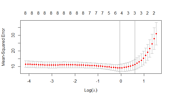
Weighted Lasso Regression in R

This line plots the cross-validated mean squared error as a function of lambda, providing insights into model performance across different regularization strengths.

Step 7: Select the lambda value based on cross-validation

R

best_lambda <- lasso_model$lambda.min
cat("Best lambda:", best_lambda, "\n")

Output:

Best lambda: 0.9518032

We extract the value of lambda that minimizes the cross-validated mean squared error and print it out.

Step 8: Fitting the model

R

lasso_fit <- glmnet(x, y, alpha = 1, weights = weights)
coefficients <- coef(lasso_fit, s = best_lambda)
print(coefficients)

Output:

10 x 1 sparse Matrix of class "dgCMatrix"
s1
(Intercept) 28.732447542
disp -0.002816656
hp -0.020557178
drat 0.572573224
wt -2.332213873
qsec .
vs 0.079748476
am .
gear .
carb .

Here, we fit the Lasso regression model using the entire dataset (`glmnet()` function) with the best lambda value obtained from cross-validation. Then, we extract and print the coefficients of the model.

Conclusion

Weighted Lasso Regression in R offers a powerful way to improve predictive modeling by considering the importance of each data point. By assigning weights to observations, this technique helps create more accurate and reliable models, especially in scenarios where some data points are more significant than others. With the help of R and packages like `glmnet`, researchers can easily implement Weighted Lasso Regression and extract valuable insights from their data. This approach opens up new possibilities for addressing real-world complexities and building more robust models for various applications.