Linear Regression Assumptions and Diagnostics using R

Linear regression is a statistical method used to model the relationship between a dependent variable and one or more independent variables. Before interpreting the results of a linear regression analysis in R, it’s important to check and ensure that the assumptions of linear regression are met. Assumptions of linear regression include linearity, independence, homoscedasticity, and normality of residuals. You can also perform various diagnostics to evaluate the model’s fit and identify potential issues. Here’s how you can perform these checks and diagnostics in the R Programming Language.

Assumptions of Linear Regression

• Linearity: The linearity assumption assumes that the relationship between the dependent variable (Y) and independent variable(s) (X) is linear. In other words, changes in X should result in constant, proportional changes in Y. To check this assumption, you can create scatterplots and evaluate the linearity of the data.
• Independence: The independence of residuals assumes that the errors (residuals) are not correlated with each other. This means that the error in one observation should be independent of the error in another. You can test this assumption using the Durbin-Watson test or by examining a plot of residuals against the order of observations.
• Homoscedasticity: Homoscedasticity means that the variance of residuals is constant across all levels of the independent variable. In other words, the spread of residuals should be roughly the same for all values of X. You can check this assumption by creating a plot of residuals against the fitted values.
• Normality of Residuals: The normality of the residuals assumption assumes that the residuals follow a normal distribution. A Q-Q plot and normality tests like the Shapiro-Wilk test can help assess this assumption.

Now, let’s walk through these assumptions with examples and explanations in R.

Linearity

R

# Load libraries and create a hypothetical dataset
library(ggplot2)
set.seed(123)
# Create individual vectors for X and Y
X <- 1:100
Y <- 2 * X + rnorm(100, mean = 0, sd = 10)

# Combine them into a data frame

data <- data.frame(X = 1:100, Y = 2 * X + rnorm(100, mean = 0, sd = 10))

# Check linearity by creating a scatterplot
ggplot(data, aes(x = X, y = Y)) + geom_point() + geom_smooth(method = "lm")

Output:

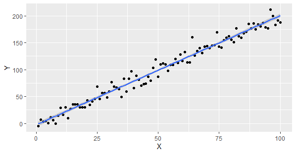
Linear Regression Assumptions and Diagnostics in R

First loads the ggplot2 library for data visualization.

• A random seed is set for reproducibility.
• Two vectors, X and Y, are created. X contains values from 1 to 100, and Y is generated as a linear function of X with added random noise.
• The X and Y vectors are combined into a data frame named data, and a scatterplot with a linear regression line is created to check for linearity between X and Y.

Independence

R

# Install and load the lmtest package
install.packages("lmtest")
library(lmtest)

# Fit the linear regression model
model <- lm(Y ~ X, data = data)

# Perform the Durbin-Watson test
dw_result <- dwtest(model)
print(dw_result)

Output:

    Durbin-Watson test
data:  model
DW = 2.2593, p-value = 0.8862
alternative hypothesis: true autocorrelation is greater than 0

Durbin-Watson Statistic (DW): The DW statistic is a measure of autocorrelation in the residuals of a regression model. The range of the statistic is between 0 and 4, where a value close to 2 suggests no significant autocorrelation. In your case, a DW statistic of approximately 2.2593 is close to 2, indicating that there is no strong evidence of autocorrelation in the residuals.

P-Value: The p-value associated with the DW statistic tests the null hypothesis that there is no autocorrelation. In your results, the p-value is approximately 0.8862. Since this p-value is greater than the common significance level of 0.05 (alpha), we fail to reject the null hypothesis. In other words, there is no significant evidence to suggest that the residuals exhibit autocorrelation.

Homoscedasticity

R

# Example: Checking homoscedasticity
# Create a plot of residuals vs. fitted values
plot(lm(Y ~ X, data = data))

Output:

Type return in the console part 4 times to get visualization of the models.

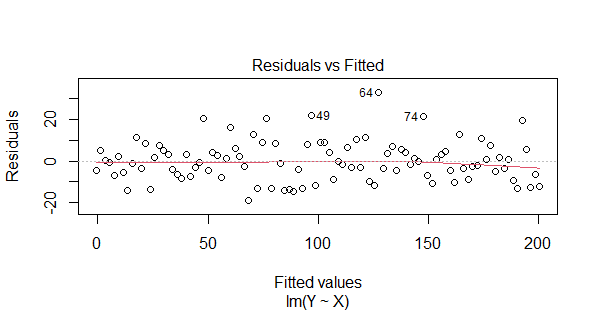
Residuals vs Fitted

• A residuals vs. fitted values plot, which is a common diagnostic plot used to assess the assumptions of a linear regression model.
• On the x-axis, you have the fitted (predicted) values from the linear regression model. On the y-axis, you have the residuals, which are the differences between the observed and predicted values.
• The plot helps check for homoscedasticity (constant variance) and linearity. If the points are randomly scattered around a horizontal line near zero, it suggests that the assumptions are met.
  
  

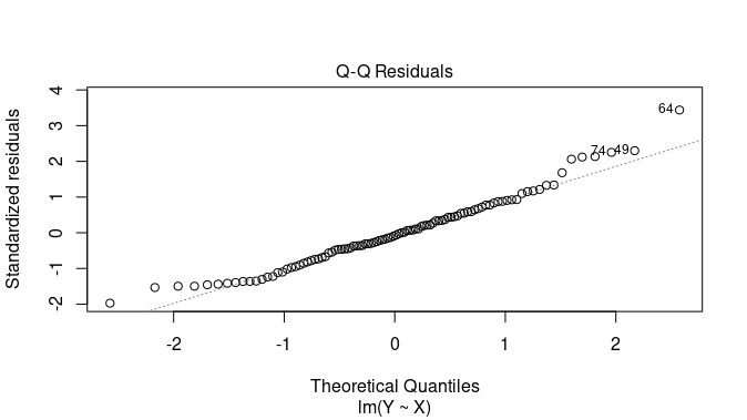
  Quantile-Quantile (Q-Q) plot

• A normal quantile-quantile (Q-Q) plot of the residuals. It is used to assess the normality of the residuals.
• If the points in this plot closely follow a straight line, it indicates that the residuals are approximately normally distributed, which is an important assumption in linear regression.
• Deviations from a straight line may suggest departures from normality.

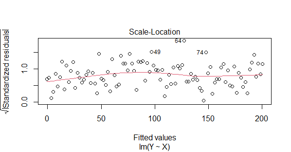
Homoscedasticity

• This plot is used to assess homoscedasticity and check for constant variance of residuals.
• The x-axis represents the fitted (predicted) values, and the y-axis shows the square root of the standardized absolute residuals.
• A spread-location plot should ideally show a horizontal line with evenly distributed points. A bow-shaped pattern suggests heteroscedasticity.

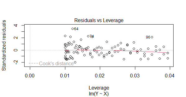
Residuals vs Leverage

• This plot is used to identify influential observations that have a high leverage and influence on the regression model.
• The x-axis typically represents the leverage values, while the y-axis shows the standardized residuals (often Cook’s distances).
• Points that are far from the center or have high Cook’s distances indicate influential observations that can heavily affect the model.
• In a well-behaved model, most points should be clustered near the center, indicating low influence.

Normality of Residuals

R

# Create a Q-Q plot of residuals
qqnorm(resid(lm(Y ~ X, data = data)))
qqline(resid(lm(Y ~ X, data = data))

Output:

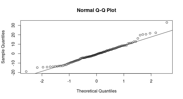
Normal Q-Q Plot

Linear Regression Diagnostics in R

Linear regression diagnostics in R are essential for assessing the validity and reliability of the linear regression model’s assumptions and for detecting potential issues that may affect the model’s performance. Below is a theoretical explanation of some common linear regression diagnostics in R.

Certainly, let’s delve into diagnostic procedures for linear regression in R. We’ll focus on the key diagnostic checks:

1. Residual Analysis: Check for patterns in the residuals.
2. Outlier Detection: Identify potential outliers.
3. Influence and Cook’s Distance: Identify influential observations.
4. Multicollinearity: Check for high correlation between predictors.

Let’s provide R code examples for each of these diagnostics using a hypothetical dataset.

R

# Example: Residual analysis
#model <- lm(Y ~ X, data = data)

# Create diagnostic plots (residuals vs. fitted values, residuals vs. normal quantiles,
#and a histogram of residuals)
par(mfrow = c(2, 2))
plot(model)

Output:

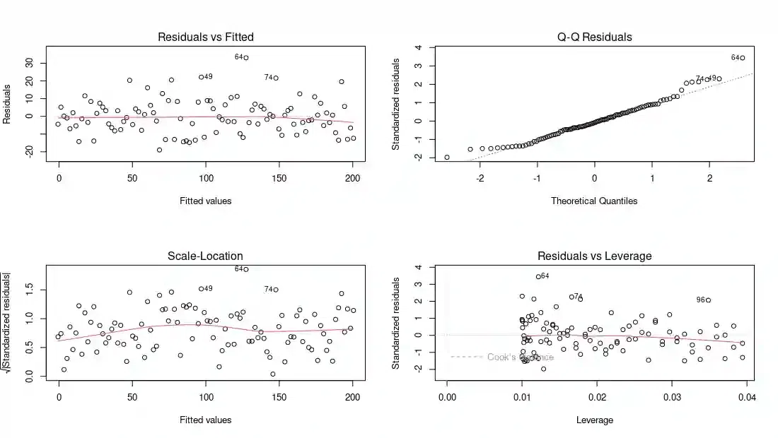
Linear Regression Diagnostics

The plot(model) function generates diagnostic plots, including residuals vs. fitted values, a Q-Q plot, and a histogram of residuals.

Outlier Detection

R

# Example: Detecting outliers
# Identify observations with high residuals
outliers <- which(abs(resid(model)) > 2 * sd(resid(model)))

# Highlight the outliers in a scatterplot
plot(data$X, data$Y)
points(data$X[outliers], data$Y[outliers], col = "red", pch = 19)

Output:

Linear Regression Assumptions and Diagnostics in R

Here, we identify outliers as observations with residuals more than two standard deviations from the mean and highlight them in a scatterplot.

Influence and Cook’s Distance

R

# Example: Influence and Cook's Distance
# Calculate Cook's distance for each observation
influential <- cooks.distance(model)

# Identify observations with Cook's distance exceeding a threshold
#(e.g., 3/n, where n is the number of observations)
threshold <- 3 / length(data$X)
influential_obs <- which(influential > threshold)

# Highlight influential observations in the scatterplot
plot(data$X, data$Y)
points(data$X[influential_obs], data$Y[influential_obs], col = "orange",
       pch = 19)

Output:

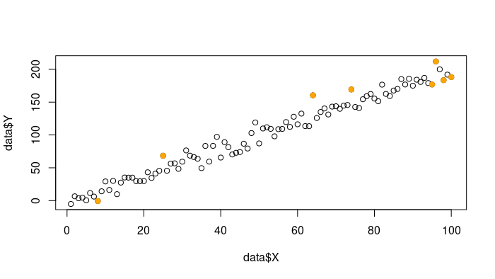
Outliers Points using Cooks Distance

This code calculates Cook’s distance for each observation and identifies influential observations with distances exceeding a threshold. These influential observations are highlighted in the scatterplot.

• To visualize the influential observations, the code plots a scatterplot of X and Y using the plot() function.
• It then highlights the influential observations by overlaying red points (colored “red”) on top of the original scatterplot. The points() function is used for this purpose, and the pch = 19 argument specifies the point character to use (a solid circle).
• The influential observations are determined by the indices identified in the previous step (stored in influential_obs), and these points are highlighted in red.

Multicollinearity

R

data(mtcars)
names(mtcars)

# Fit the linear regression model
vif_model <- lm(mpg ~ cyl + disp + hp, data = mtcars)

# Check for multicollinearity by calculating the variance inflation factor (VIF)
library(car)
vif_values <- vif(vif_model)

# Print the VIF values for each predictor
print(vif_values)

Output:

     cyl     disp       hp 
6.732984 5.521460 3.350964 

We use the vif() function from the car package to calculate VIF values for each predictor. High VIF values indicate potential multicollinearity issues.