Understanding Gradient Clipping

Gradient Clipping is the process that helps maintain numerical stability by preventing the gradients from growing too large. When training a neural network, the loss gradients are computed through backpropagation. However, if these gradients become too large, the updates to the model weights can also become excessively large, leading to numerical instability. This can result in the model producing NaN (Not a Number) values or overflow errors, which can be problematic. This problem is often referred to as ‘gradient exploding’, it could be solved by clipping the gradient to the value that we want it to be. Let’s thoroughly discuss gradient clipping.

Gradient Clipping in Deep Learning

Gradient Clipping is a technique used during the training of neural networks to address the issue of exploding gradients. When the gradients of the loss function concerning the parameters become too large, it can cause the model’s weights to be updated by huge amounts, leading to numerical instability and a slow or even halted convergence of the training process. By using Gradient Clipping, we can maintain numerical stability by preventing the gradients from growing too large, thus improving the model’s overall performance.

Gradient clipping is a very effective technique that helps address the exploding gradient problem during training. By limiting the magnitude of the gradients, it helps to prevent them from growing unchecked and becoming too large. This ensures that the model learns more effectively and prevents it from getting stuck in a local minima. The clip value or clip threshold is an important parameter that determines how aggressively the gradients are scaled down.

How does Gradient Clipping work?

Let’s discuss the step-by-step description of gradient clipping:

1. Calculate Gradients:
   When the model is learning, it’s like a student taking an exam. Backpropagation is like a teacher grading the exam and giving feedback to the student. It calculates the gradients of the model’s parameters with respect to the loss function, helping the model learn and improve its performance. So, think of backpropagation as a helpful teacher guiding the model to success!
   
2. Compute Gradient Norm:
   To measure the magnitude of the gradients, we can use different types of norms such as the L2 norm (also known as the Euclidean norm) or the L1 norm. These norms help us to quantify the size of the gradients and understand how fast the parameters are changing. The L2 norm calculates the square root of the sum of the squares of the individual gradients, while the L1 norm calculates the sum of the absolute values of the gradients. By measuring the norm of the gradients, we can monitor the training process and adjust the learning rate accordingly to ensure that the model is converging efficiently.
   
3. Clip Gradients:
   If the computed gradient norm exceeds the predefined clip threshold, the gradients are scaled down to ensure that the norm does not exceed this threshold. The scaling factor is determined by dividing the clip threshold by the gradient norm.
   • 
   • The clipped gradients become, .
     
4. Update Model Parameters:
   The clipped gradients are used to update the model parameters. By using the clipped gradients to update the model parameters, we can prevent the weights from being updated by excessively large amounts, which can lead to numerical instability and slow down the training process. This helps to ensure that the model is learning effectively and converging towards a good solution.

The clip_threshold discussed here is a type of hyperparameter whose value could be determined by experimenting on the dataset present in front of us.

Types of Gradient Clipping Techniques

There are two different gradient clipping techniques that are used, gradient clipping by value and gradient clipping by norm, let’s discuss them thoroughly.

Clipping by Value:

‘Clipping by value’ is the most straightforward and effective gradient clipping technique, in this method the gradients are individually clipped so that they lie in the predefined range that is mentioned. This technique is done elementwise, so each component of the gradient vector is clipped individually. In this gradient clipping technique, the minimum and maximum thresholds are defined, and the range is set accordingly so that the gradient’s value lies in between the minimum and maximum value.

After the computation of the gradients through backpropagation, inspection of the gradient component is done, if the gradient component is greater than the maximum threshold it’s value is set to maximum threshold and if the gradient component is lower than the minimum threshold value mentioned then the value of the gradient component is set to minimum threshold value and if the value of the gradient component lies in between the range of minimum and maximum threshold value then the gradient component is set as it is and not changed.

Clipping by Norm:

In the ‘clipping by norm’ technique of gradient clipping the gradients are clipped if their norm (or their size) is greater than the specified threshold value. In contrast to the ‘clipping by value’ here in this case the values of the gradients greater than or less than the threshold values are not set to the threshold values. It makes sure that the norm of the updated gradients remains small and manageable, and the learning process is more stable. There are different types of ‘clipping by norm’ techniques let’s explore them one by one.

• L2 Norm Clipping:
  In this form of norm clipping technique the gradient value is clipped down if it’s L2 norm (Euclidean norm) exceeds the predefined threshold value. The L2 norm or the Euclidean norm is calculated as the square root of the squared values of its components. Considering gradient vector as g = [] where is the gradient with respect to the parameter of the model and n is the total number of model parameters. Therefore, the L2 norm is represented as:
  
  Now, if the L2 norm exceeds the threshold value the upgraded gradient after clipping of the components becomes:
  
• L1 Norm Clipping:
  L1 norm technique of gradient is similar to the L2 norm gradient clipping technique, in this technique if the L1 norm exceeds the threshold that we defined in alignment with our specific requirements. L1 norm of a gradient is the sum of the absolute values of all its components. Therefore, the L1 norm is represented as:
  
  If the L1 norm exceeds the threshold value, the upgraded gradient after clipping becomes:
  

Gradient clipping by norm provides a more global control over the gradients, and it is often used to address the exploding gradient problem.

Necessity of Gradient Clipping

Gradient Clipping is a crucial step in the training of neural networks since it helps in addressing the issue of exploding gradients. The exploding gradients problem arises when the gradients in the backpropagation process becomes excessively large in value, causing instability in training of model. Now we will see some of the most important points which explains the necessity of gradient clipping in neural network model training.

1. Stability of Training: During the training of neural network, the optimization algorithm adjusts the value of model parameters with the help of obtained gradients. If the gradients are obtained to be too large the weights of the model updates by a large value causing the model to oscillate and diverge instead of converging to an optimal solution. Whereas gradient clipping limits the size of the gradient and eliminating this issue of instability in the model.
2. Improving Generalization: Large gradients might cause the model to overfit to the training data, which in turn might capture more noise and makes the model bad at generalization. Gradient clipping removes this hindrance and makes the model generalize better on new data preventing extreme updates.
3. Convergence to Optimal Solution: Exploding gradient prevents the model to converge to optimal solution and instead produces more unstable modelling of data. By clipping the gradient values, we can suspend the possibility of instability, the model gets better at navigating the parameter space enabling consistent progress toward optimal solution.
4. Compatibility with Activation Function: Some of the activation functions such as ‘Sigmoid’ and ‘tanh’ functions are sensitive to large input. Gradient clipping ensures the gradient passed through the activation function is within a reasonable range which also helps in removing undesirable behavior like saturation.
5. Mitigating Vanishing Gradient Problem: Sometimes the gradient of the loss function with respect to the weights become extremely small which causes the weight to stop updating or even halt the process of training the model. Norm-based gradient clipping helps in preventing the vanishing gradient problem by maintaining the range of value for the gradient that is effective for training the model.
   

Gradient clipping is a necessary and effective technique to ensure the stability, reliability, and numerical robustness of the training process in neural networks.

Gradient Clipping on Real World Example Dataset

Let’s apply gradient clipping on IMDB dataset for sentiment analysis and see if it improves the performance:

1. Importing Libraries

We will be importing necessary libraries from TensorFlow. TensorFlow is a popular machine learning library, and Keras is its high-level API for building and training deep learning models. We will also be importing the Matplotlib library for the before and after gradient clipping visualization.

Python3

import tensorflow as tf
from tensorflow.keras.models import Sequential
from tensorflow.keras.layers import Embedding, LSTM, Dense
import matplotlib.pyplot as plt

2. Loading and Preparing the IMDB Dataset

The IMDb dataset is a popular dataset for sentiment analysis, which consists of movie reviews labeled as positive or negative. In TensorFlow, the dataset can be loaded using the dataset utility, with the num_words parameter set to a specific value (e.g. num_words=10000) to keep only the top 10,000 most frequent words in the dataset. This helps to reduce the number of words in the dataset and make the analysis more manageable. After loading the dataset, the sequences (reviews) are padded with zeros or truncated to ensure they have the same length, which is necessary for feeding the data into a neural network. This step helps to ensure that all the inputs to the neural network have the same shape, which is important for efficient training.

Python3

(x_train, y_train), (x_test, y_test) = tf.keras.datasets.imdb.load_data(num_words=10000)
x_train = tf.keras.preprocessing.sequence.pad_sequences(x_train, maxlen=100)
x_test = tf.keras.preprocessing.sequence.pad_sequences(x_test, maxlen=100)

3. Model Building Function

The build_model function is responsible for constructing the neural network model for sentiment analysis. The function includes an Embedding layer, which maps each word in the input sequence to a high-dimensional vector space, an LSTM (Long Short-Term Memory) layer, which can capture long-term dependencies in the input sequence, and a Dense layer with a sigmoid activation function for binary classification. The function takes a parameter apply_clipping, which determines whether to apply gradient clipping during training. If apply_clipping is set to True, the Adam optimizer is configured with clipvalue=1.0. This limits the gradients during training to the range [-1, 1].

Python3

def build_model(apply_clipping=False):
    # Model architecture
    model = Sequential([
        Embedding(input_dim=10000, output_dim=32, input_length=100),
        LSTM(100),
        Dense(1, activation='sigmoid')
    ])

    # Configure optimizer with gradient clipping
    if apply_clipping:
        optimizer = tf.keras.optimizers.Adam(clipvalue=1.0)
    else:
        optimizer = 'adam'

    model.compile(optimizer=optimizer, loss='binary_crossentropy', metrics=['accuracy'])
    return model

4. Model Training

In the sentiment analysis, two models are trained on the IMDB dataset – one with gradient clipping (model_with_clipping) and one without (model_without_clipping). Both models are trained for 5 epochs with a batch size of 64. During training, the model_with_clipping applies gradient clipping to prevent the gradients from becoming too large, which can lead to numerical instability and slow down the training process. The model_without_clipping, on the other hand, does not apply gradient clipping and relies on the default behavior of the Adam optimizer.

Python3

model_without_clipping = build_model(apply_clipping=False)
history_without_clipping = model_without_clipping.fit(x_train, y_train, epochs=5, batch_size=64, validation_split=0.2)

model_with_clipping = build_model(apply_clipping=True)
history_with_clipping = model_with_clipping.fit(x_train, y_train, epochs=5, batch_size=64, validation_split=0.2)

Output:

Epoch 1/5
313/313 [==============================] - 14s 40ms/step - loss: 0.4437 - accuracy: 0.7833 - val_loss: 0.3428 - val_accuracy: 0.8508
Epoch 2/5
313/313 [==============================] - 13s 42ms/step - loss: 0.2697 - accuracy: 0.8935 - val_loss: 0.3490 - val_accuracy: 0.8458
Epoch 3/5
313/313 [==============================] - 17s 54ms/step - loss: 0.2058 - accuracy: 0.9228 - val_loss: 0.3772 - val_accuracy: 0.8466
Epoch 4/5
313/313 [==============================] - 15s 49ms/step - loss: 0.1709 - accuracy: 0.9370 - val_loss: 0.4207 - val_accuracy: 0.8378
Epoch 5/5
313/313 [==============================] - 16s 50ms/step - loss: 0.1248 - accuracy: 0.9568 - val_loss: 0.4753 - val_accuracy: 0.8306
Epoch 1/5
313/313 [==============================] - 17s 51ms/step - loss: 0.4502 - accuracy: 0.7868 - val_loss: 0.3799 - val_accuracy: 0.8422
Epoch 2/5
313/313 [==============================] - 15s 49ms/step - loss: 0.2691 - accuracy: 0.8935 - val_loss: 0.3545 - val_accuracy: 0.8428
Epoch 3/5
313/313 [==============================] - 16s 51ms/step - loss: 0.2180 - accuracy: 0.9158 - val_loss: 0.4229 - val_accuracy: 0.8360
Epoch 4/5
313/313 [==============================] - 16s 52ms/step - loss: 0.1723 - accuracy: 0.9376 - val_loss: 0.4262 - val_accuracy: 0.8314
Epoch 5/5
313/313 [==============================] - 16s 52ms/step - loss: 0.1328 - accuracy: 0.9550 - val_loss: 0.5689 - val_accuracy: 0.8240

5. Results Visualization

After training both models, the training history is plotted using Matplotlib to compare the performance of the models with and without gradient clipping. The plot_history function is used to create plots for both the training loss and accuracy.

Python3

def plot_history(histories, key='loss'):
    plt.figure(figsize=(16, 10))

    for name, history in histories:
        val = plt.plot(history.epoch, history.history['val_'+key],
                       '--', label=name.title() + ' Val')
        plt.plot(history.epoch, history.history[key], color=val[0].get_color(),
                 label=name.title() + ' Train')

    plt.xlabel('Epochs')
    plt.ylabel(key.replace('_', ' ').title())
    plt.legend()

    plt.xlim([0, max(history.epoch)])

# Plotting loss and accuracy
plot_history([('Without Clipping', history_without_clipping),
              ('With Clipping', history_with_clipping)],
             key='loss')

plot_history([('Without Clipping', history_without_clipping),
              ('With Clipping', history_with_clipping)],
             key='accuracy')

Output:

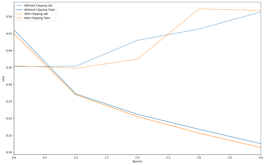
Loss with respect to epoch before vs after gradient clipping

Here in the above output plot, the dotted blue line represents the loss on validation set without gradient clipping, the dotted orange line represents the loss on validation set after gradient clipping, the blue line represents loss on training set without clipping and the orange line represents loss on training set with gradient clipping.

Accuracy with respect to epoch before vs after gradient clipping

Here, in the above plot, the dotted blue line represents accuracy on validation set without gradient clipping, the dotted orange line represents accuracy on validation set with gradient clipping, the blue line represents accuracy on training set without gradient clipping and the orange line represents accuracy on training set with gradient clipping.

By comparing the training history of the models with and without gradient clipping, we can visually see how the addition of gradient clipping affects the performance of the model. Overall, the plot_history function is an important part of the sentiment analysis pipeline, as it helps to visualize the training history and identify any issues with the model’s performance.