Stochastic Gradient Descent Classifier

One essential tool in the data science and machine learning toolkit for a variety of classification tasks is the stochastic gradient descent (SGD) classifier. Through an exploration of its functionality and critical role in data-driven decision-making, we set out to explore the complexities of the SGD Classifier in this article.

A flexible classification technique that shares close ties with the SGD Regressor is the SGD Classifier. It works by progressively changing model parameters in the direction of a loss function’s sharpest gradient. Its capacity to update these parameters with a randomly chosen subset of the training data for every iteration is what distinguishes it as “stochastic”. The SGD Classifier is a useful tool because of its versatility, especially in situations where real-time learning is required and big datasets are involved. We will examine the fundamental ideas of the SGD Classifier in this post, dissecting its key variables and hyperparameters. We will also discuss any potential drawbacks and examine its benefits, such as scalability and efficiency. You will have a thorough grasp of the SGD Classifier and its crucial role in the field of data-driven decision-making by the time this journey is over.

Stochastic Gradient Descent

One popular optimization method in deep learning and machine learning is stochastic gradient descent (SGD). Large datasets and complicated models benefit greatly from its training. To minimize a loss function, SGD updates model parameters iteratively. It differentiates itself as “stochastic” by employing mini-batches, or random subsets, of the training data in each iteration, which introduces a degree of randomness while maximizing computational efficiency. By accelerating convergence, this randomness can aid in escaping local minima. Modern machine learning algorithms rely heavily on SGD because, despite its simplicity, it may be quite effective when combined with regularization strategies and suitable learning rate schedules.

How Stochastic Gradient Descent Works?

Here’s how the SGD process typically works:

• Initialize the model parameters randomly or with some default values.
• Randomly shuffle the training data.
• For each training example: Compute the gradient of the cost function with respect to the current model parameters using the current example.
• Update the model parameters in the direction of the negative gradient by a small step size known as the learning rate.
• Repeat this process for a specified number of iterations (epochs).

Stochastic Gradient Descent Algorithm

For machine learning model training, initializing model parameters (θ) and selecting a low learning rate (α) are the first steps in performing stochastic gradient descent (SGD). Next, to add unpredictability, the training data is jumbled at random. Every time around, the algorithm analyzes a single training sample and determines the cost function‘s gradient (J) in relation to the model’s parameters. The size and direction of the steepest slope are represented by this gradient. The model is adjusted to minimize the cost function and provide predictions that are more accurate by updating θ in the gradient’s opposite direction. The model can efficiently learn from and adjust to new information by going through these iterative processes for every data point.

The cost function,, is typically a function of the difference between the predicted value and the actual target . In regression problems, it’s often the mean squared error; in classification problems, it can be cross-entropy loss, for example.

For Regression (Mean Squared Error):

Cost Function:

Gradient (Partial Derivatives):

Update Parameters

Update the model parameters (θ) based on the gradient and the learning rate:

where,

• θ: Updated model parameters.
• α: Learning rate.
• ∇J(θ): Gradient vector computed.

What is the SGD Classifier?

The SGD Classifier is a linear classification algorithm that aims to find the optimal decision boundary (a hyperplane) to separate data points belonging to different classes in a feature space. It operates by iteratively adjusting the model’s parameters to minimize a cost function, often the cross-entropy loss, using the stochastic gradient descent optimization technique.

How it Differs from Other Classifiers:

The SGD Classifier differs from other classifiers in several ways:

• Stochastic Gradient Descent: Unlike some classifiers that use closed-form solutions or batch gradient descent (which processes the entire training dataset in each iteration), the SGD Classifier uses stochastic gradient descent. It updates the model’s parameters incrementally, processing one training example at a time or in small mini-batches. This makes it computationally efficient and well-suited for large datasets.
• Linearity: The SGD Classifier is a linear classifier, meaning it constructs a linear decision boundary to separate classes. This makes it suitable for problems where the relationship between features and the target variable is approximately linear. In contrast, algorithms like decision trees or support vector machines can capture more complex decision boundaries.
• Regularization: The SGD Classifier allows for the incorporation of L1 or L2 regularization to prevent overfitting. Regularization terms are added to the cost function, encouraging the model to have smaller parameter values. This is particularly useful when dealing with high-dimensional data.

Common Use Cases in Machine Learning

The SGD Classifier is commonly used in various machine learning tasks and scenarios:

1. Text Classification: It’s often used for tasks like sentiment analysis, spam detection, and text categorization. Text data is typically high-dimensional, and the SGD Classifier can efficiently handle large feature spaces.
2. Large Datasets: When working with extensive datasets, the SGD Classifier’s stochastic nature is advantageous. It allows you to train on large datasets without the need to load the entire dataset into memory, making it memory-efficient.
3. Online Learning: In scenarios where data streams in real-time, such as clickstream analysis or fraud detection, the SGD Classifier is well-suited for online learning. It can continuously adapt to changing data patterns.
4. Multi-class Classification: The SGD Classifier can be used for multi-class classification tasks by extending the binary classification approach to handle multiple classes, often using the one-vs-all (OvA) strategy.
5. Parameter Tuning: The SGD Classifier is a versatile algorithm that can be fine-tuned with various hyperparameters, including the learning rate, regularization strength, and the type of loss function. This flexibility allows it to adapt to different problem domains.

Parameters of Stochastic Gradient Descent Classifier

Stochastic Gradient Descent (SGD) Classifier is a versatile algorithm with various parameters and concepts that can significantly impact its performance. Here’s a detailed explanation of some of the key parameters and concepts relevant to the SGD Classifier:

1. Learning Rate (α):

• The learning rate (α) is a crucial hyperparameter that determines the size of the steps taken during parameter updates in each iteration.
• It controls the trade-off between convergence speed and stability.
• A larger learning rate can lead to faster convergence but may result in overshooting the optimal solution.
• In contrast, a smaller learning rate may lead to slower convergence but with more stable updates.
• It’s important to choose an appropriate learning rate for your specific problem.

2. Batch Size:

The batch size defines the number of training examples used in each iteration or mini-batch when updating the model parameters. There are three common choices for batch size:

• Stochastic Gradient Descent (batch size = 1): In this case, the model parameters are updated after processing each training example. This introduces significant randomness and can help escape local minima but may result in noisy updates.
• Mini-Batch Gradient Descent (1 < batch size < number of training examples): Mini-batch SGD strikes a balance between the efficiency of batch gradient descent and the noise of stochastic gradient descent. It’s the most commonly used variant.
• Batch Gradient Descent (batch size = number of training examples): In this case, the model parameters are updated using the entire training dataset in each iteration. While this can lead to more stable updates, it is computationally expensive, especially for large datasets.

3. Convergence Criteria:

Convergence criteria are used to determine when the optimization process should stop. Common convergence criteria include:

• Fixed Number of Epochs: You can set a predefined number of epochs, and the algorithm stops after completing that many iterations through the dataset.
• Tolerance on the Change in the Cost Function: Stop when the change in the cost function between consecutive iterations becomes smaller than a specified threshold.
• Validation Set Performance: You can monitor the performance of the model on a separate validation set and stop training when it reaches a satisfactory level of performance.

4. Regularization (L1 and L2):

• Regularization is a technique used to prevent overfitting.
• The SGD Classifier allows you to incorporate L1 (Lasso) and L2 (Ridge) regularization terms into the cost function.
• These terms add a penalty based on the magnitude of the model parameters, encouraging them to be small.
• The regularization strength hyperparameter controls the impact of regularization on the optimization process.

5. Loss Function:

• The choice of the loss function determines how the classifier measures the error between predicted and actual class labels.
• For binary classification, the cross-entropy loss is commonly used, while for multi-class problems, the categorical cross-entropy or softmax loss is typical.
• The choice of the loss function should align with the problem and the activation function used.

6. Momentum and Adaptive Learning Rates:

To enhance convergence and avoid oscillations, you can use momentum techniques or adaptive learning rates. Momentum introduces an additional parameter that smoothers the updates and helps the algorithm escape local minima. Adaptive learning rate methods automatically adjust the learning rate during training based on the observed progress.

7. Early Stopping:

Early stopping is a technique used to prevent overfitting. It involves monitoring the model’s performance on a validation set during training and stopping the optimization process when the performance starts to degrade, indicating overfitting.

Python Code using SGD to classify the famous Iris Dataset

To implement a Stochastic Gradient Descent Classifier in Python, you can follow these steps:

Installing Required Libraries

!pip install numpy
!pip install scikit-learn
!pip install matplotlib

You will need to import libraries such as NumPy for numerical operations, Scikit-Learn for machine learning tools and Matplotlib for data visualization.

Importing Required Libraries

Python3

# importing Libraries
import numpy as np
import matplotlib.pyplot as plt
from sklearn.datasets import load_iris
from sklearn.model_selection import train_test_split
from sklearn.linear_model import SGDClassifier
from sklearn.metrics import accuracy_score, confusion_matrix, classification_report
import seaborn as sns

This code loads the Iris dataset, imports the required libraries for a machine learning classification task, splits the training and testing phases, builds an SGD Classifier, assesses the model’s accuracy, produces a confusion matrix, a classification report, and displays the data with scatter plots and a heatmap for the confusion matrix.

Load and Prepare Data

Python3

# Load the Iris dataset
data = load_iris()
X, y = data.data, data.target

# Split the data into training and testing sets
X_train, X_test, y_train, y_test = train_test_split(
    X, y, test_size=0.3, random_state=42)

This code loads the Iris dataset, which is made up of target labels in y and features in X. The data is then split 70–30 for training and testing purposes, with a reproducible random seed of 42. This yields training and testing sets for both features and labels.

Create an SGD Classifier

Python3

# Create an SGD Classifier
clf = SGDClassifier(loss='log_loss', alpha=0.01,
                    max_iter=1000, random_state=42)

An SGD Classifier (clf) is instantiated for classification tasks in this code. Because the classifier is configured to use the log loss (logistic loss) function, it can be used for both binary and multiclass classification. Furthermore, to help avoid overfitting, L2 regularization is used with an alpha parameter of 0.01. To guarantee consistency of results, a random seed of 42 is chosen, and the classifier is programmed to run up to 1000 iterations during training.

Train the Classifier and make Predictions

Python3

# Train the classifier
clf.fit(X_train, y_train)

# Make predictions
y_pred = clf.predict(X_test)

Using the training data (X_train and y_train), these lines of code train the SGD Classifier (clf). Following training, the model is applied to generate predictions on the test data (X_test), which are then saved in the y_pred variable for a future analysis.

Evaluate the Model

Python3

# Evaluate the model
accuracy = accuracy_score(y_test, y_pred)
print(f'Accuracy: {accuracy}')

Output:

Accuracy: 0.9555555555555556

These lines of code compare the predicted labels (y_pred) with the actual labels of the test data (y_test) to determine the classification accuracy. To assess the performance of the model, the accuracy score is displayed on the console.

Confusion Matrix

Python3

# Plot the confusion matrix using Seaborn
plt.figure(figsize=(6, 6))
sns.heatmap(conf_matrix, annot=True, fmt="d", cmap="Blues", cbar=False,
            xticklabels=data.target_names, yticklabels=data.target_names)
plt.xlabel('Predicted')
plt.ylabel('Actual')
plt.title('Confusion Matrix')
plt.show()

Output:

Confusion Matrix

With the help of the Seaborn library, these lines of code visualize the confusion matrix as a heatmap. The counts of true positive, true negative, false positive, and false negative predictions are all included in the conf_matrix. The values are labeled on the heatmap, and the target class names are set for the x and y labels. At last, the plot gets a title, which is then shown. Understanding the model’s performance in each class is made easier with the help of this representation.

Scatter Plot for two classes(Setosa and Versicolor)

Python3

# Visualize the Sepal length vs. Sepal width for two classes (Setosa and Versicolor)
plt.figure(figsize=(8, 6))
plt.scatter(X[y == 0, 0], X[y == 0, 1], label="Setosa", marker="o")
plt.scatter(X[y == 1, 0], X[y == 1, 1], label="Versicolor", marker="x")
plt.xlabel("Sepal Length (cm)")
plt.ylabel("Sepal Width (cm)")
plt.legend()
plt.title("Iris Dataset: Sepal Length vs. Sepal Width")
plt.show()

Output:

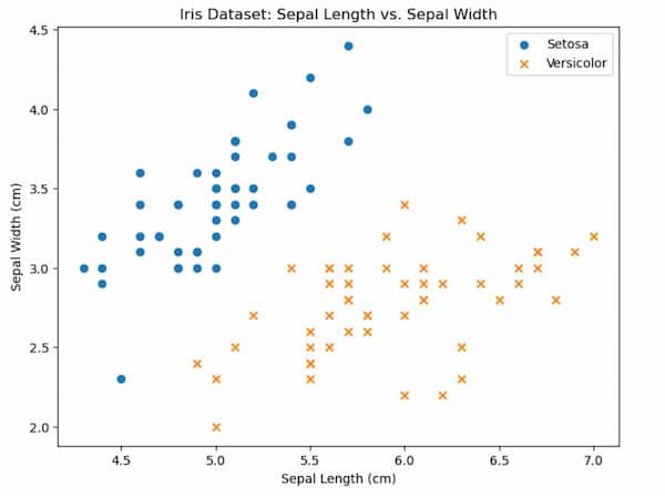
Scatter Plot

For the two classes Setosa and Versicolor in the Iris dataset, this code generates a scatter plot to show the relationship between Sepal Length and Sepal Width. Plotting the data points for each class with unique markers (circles for Setosa and crosses for Versicolor) is done using the plt.scatter function. To enhance the plot’s visual appeal and informativeness, x and y-axis labels, a legend, and a title are added.

Classification report

Python3

# Print the classification report
class_names = data.target_names
report = classification_report(y_test, y_pred, target_names=class_names)
print("Classification Report:\n", report)

Output:

Classification Report:
               precision    recall  f1-score   support

      setosa       1.00      1.00      1.00        19
  versicolor       1.00      0.85      0.92        13
   virginica       0.87      1.00      0.93        13

    accuracy                           0.96        45
   macro avg       0.96      0.95      0.95        45
weighted avg       0.96      0.96      0.96        45

Using the classification_report function, this code generates the classification report for the actual labels (y_test) and the predicted results (y_pred), which includes multiple classification metrics including precision, recall, F1-score, and support. A summary of the model’s classification performance is printed in the report along with the target class names from the Iris dataset.

Advantages of SGD Classifier

The Stochastic Gradient Descent (SGD) classifier offers several advantages:

• Efficiency with Large Datasets: One of the most significant advantages of the SGD Classifier is its efficiency with large datasets. Since it processes one training example at a time or small mini-batches, it doesn’t require the entire dataset to be loaded into memory. This makes it suitable for scenarios with massive amounts of data.
• Online Learning: SGD is well-suited for online learning, where the model can adapt and learn from incoming data streams in real-time. It can continuously update its parameters, making it useful for applications like recommendation systems, fraud detection, and clickstream analysis.
• Quick Convergence: SGD often converges faster than batch gradient descent because of the more frequent parameter updates. This speed can be beneficial when you have computational constraints or want to quickly iterate through different model configurations.
• Regularization Support: The SGD Classifier allows for the incorporation of L1 and L2 regularization terms, which help prevent overfitting. These regularization techniques are useful when dealing with high-dimensional data or when you need to reduce the complexity of the model.

Disadvantages of SGD Classifier

The Stochastic Gradient Descent (SGD) Classifier has some disadvantages and limitations:

• Stochastic Nature: The stochastic nature of SGD introduces randomness in parameter updates, which can make the convergence path noisy. It may lead to slower convergence on some iterations or even convergence to suboptimal solutions.
• Tuning Learning Rate: Selecting an appropriate learning rate is crucial but can be challenging. If the learning rate is too high, the algorithm may overshoot the optimal solution, while too low of a learning rate can lead to slow convergence. Finding the right balance can be time-consuming.
• Sensitivity to Feature Scaling: SGD is sensitive to feature scaling. Features should ideally be standardized (i.e., mean-centered and scaled to unit variance) to ensure optimal convergence. Failure to do so can lead to convergence issues.
• Limited Modeling Capabilities: Being a linear classifier, the SGD Classifier may struggle with complex data that doesn’t have a linear decision boundary. In such cases, other algorithms like decision trees or neural networks might be more suitable.

Conclusion

In summary, the Stochastic Gradient Descent (SGD) Classifier in Python is a versatile optimization algorithm that underpins a wide array of machine learning applications. By efficiently updating model parameters using random subsets of data, SGD is instrumental in handling large datasets and online learning. From linear and logistic regression to deep learning and reinforcement learning, it offers a powerful tool for training models effectively. Its practicality, broad utility, and adaptability continue to make it a cornerstone of modern data science and machine learning, enabling the development of accurate and efficient predictive models across diverse domains.