Twitter Sentiment Analysis on Russia-Ukraine War Using Python

In this article, we are going to see how we can perform the Twitter sentiment analysis on the Russia-Ukraine War using Python.

Twitter Sentiment Analysis on Russia-Ukraine War

The role of social media in public opinion has been profound and evident since it started gaining attention. Social media allows us to share information in a great capacity and on a grand scale. Just after the news of a possible Russia-Ukraine war, netizens from across the globe started flooding the platform with their opinions. Analysis of these opinions can help us to understand the thinking of the public on different events before and during the war. We take tweets with search keywords related to the Russian invasion of Ukraine like #UkraineWar #RussiaInvade #StandwithUkraine #UkraineNATO etc. from January 2022 to the first week of March 2022 with the aim is to understanding the sentiment of people from all over the world during these events.

First, to analyze the sentiment and process the data, we will need to import the following dependencies:

Importing Dependencies

First, we will need the following dependencies to be imported.

Python3

# Import Libraries

from textblob import TextBlob
import sys
import matplotlib.pyplot as plt
import pandas as pd
import numpy as np
import os
import nltk
import re
import string
import seaborn as sns


from PIL import Image
from nltk.sentiment.vader import SentimentIntensityAnalyzer
from nltk.stem import SnowballStemmer
from nltk.sentiment.vader import SentimentIntensityAnalyzer
from sklearn.feature_extraction.text import CountVectorizer

Dataset Loading

The dataset used consists of tweets from the Russia-Ukraine war, spanning a period of 65 days. it is having tweets from 1st January 2022 to 6th March 2022. This timeline includes the pre and peak of the invasion period. This dataset contains a maximum of 5000 tweets per day with the following search keywords ‘Ukraine war’, ‘Ukraine troops’, ‘Ukraine border’, ‘Ukraine NATO’, ‘StandwithUkraine’, ‘Russian troops’, ‘Russian border Ukraine’, ‘Russia invade’. The dataset is divided into 8 Comma-separated values (CSV) files based on the search keyword. The files are extracted and loaded using Pandas Dataframe. The code for loading the dataset will be:

Python3

# List of file paths
file_paths = [
    "/ukraine-war-tweets-dataset-65-days/Russia_invade.csv",
    "/ukraine-war-tweets-dataset-65-days/Russian_border_Ukraine.csv",
    "/ukraine-war-tweets-dataset-65-days/Russian_troops.csv",
    "/ukraine-war-tweets-dataset-65-days/StandWithUkraine.csv",
    "/ukraine-war-tweets-dataset-65-days/Ukraine_border.csv",
    "/ukraine-war-tweets-dataset-65-days/Ukraine_nato.csv",
    "/ukraine-war-tweets-dataset-65-days/Ukraine_troops.csv",
    "/ukraine-war-tweets-dataset-65-days/Ukraine_war.csv"
]

# Load all CSV files into a single DataFrame
tweets = pd.concat([pd.read_csv(file) for file in file_paths], ignore_index=True)

So, here we have loaded all the 8 CSV files in a Pandas Dataframe.

Removing Duplicates

Then the most important thing was to remove any duplicate tweets from the dataset. Below codes helps us to do so –

Python3

tweets.drop_duplicates(inplace=True)  # remove duplicates

Preprocessing

The date column present in the dataset has both date and time. For the next processing steps, it is helpful to remove the time portion for it. Below codes will help to do so –

Python3

# slicing the date , and removing the time portion
tweets['date'] = tweets.date.str.slice(0, 10)

Now, we have tweets are in 61 different languages for 65 days. To check that we can use the following codes –

Python3

# checking all the unique dates in the dataset
print(tweets['date'].unique())  

# checking how many unique language
# tweets are present in the dataset
print(tweets["lang"].unique())

Output:

['2022-03-05' '2022-03-04' '2022-03-03' '2022-03-02' '2022-03-01'
 '2022-02-28' '2022-02-27' '2022-02-26' '2022-02-25' '2022-02-24'
 '2022-02-23' '2022-02-22' '2022-02-21' '2022-02-20' '2022-02-19'
 '2022-02-18' '2022-02-17' '2022-02-16' '2022-02-15' '2022-02-14'
 '2022-02-13' '2022-02-12' '2022-02-11' '2022-02-10' '2022-02-09'
 '2022-02-08' '2022-02-07' '2022-02-06' '2022-02-05' '2022-02-04'
 '2022-02-03' '2022-02-02' '2022-02-01' '2022-01-31' '2022-01-30'
 '2022-01-29' '2022-01-28' '2022-01-27' '2022-01-26' '2022-01-25'
 '2022-01-24' '2022-01-23' '2022-01-22' '2022-01-21' '2022-01-20'
 '2022-01-19' '2022-01-18' '2022-01-17' '2022-01-16' '2022-01-15'
 '2022-01-14' '2022-01-13' '2022-01-12' '2022-01-11' '2022-01-10'
 '2022-01-09' '2022-01-08' '2022-01-07' '2022-01-06' '2022-01-05'
 '2022-01-04' '2022-01-03' '2022-01-02' '2022-01-01' '2021-12-31']

['en' 'pt' 'zh' 'nl' 'it' 'es' 'de' 'ca' 'cy' 'fr' 'tr' 'ro' 'pl' 'cs'
 'ja' 'in' 'hi' 'und' 'sv' 'tl' 'et' 'fi' 'da' 'no' 'el' 'ht' 'ru' 'ar'
 'ko' 'fa' 'sl' 'iw' 'dv' 'ta' 'lv' 'pa' 'eu' 'kn' 'ur' 'bn' 'gu' 'uk'
 'ne' 'ml' 'sd' 'hu' 'lt' 'my' 'vi' 'te' 'th' 'ka' 'is' 'sr' 'bg' 'am'
 'mr' 'si' 'km' 'or' 'ps']

Now we will take only English tweets and remove all the non-English tweets. The below code snippet will help us to do so –

Python3

# before removing the non-english tweets
print(tweets.shape)

# removing all the tweets expect the
# non-english tweets
tweets = tweets[tweets['lang'] == 'en']
print("After removing non-english Tweets")

# only the number of english tweets
print(tweets.shape)  

Output:

(1313818, 29)
After removing non-english Tweets
(1204218, 29)

Here, we can find earlier we had 1313818 tweets and after removing the non-English tweets we are having 1204218 tweets.

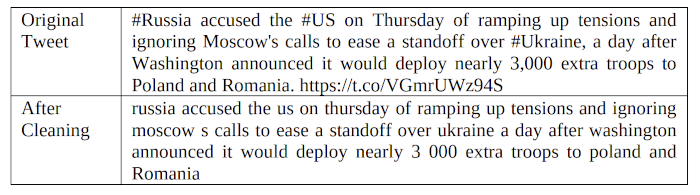
Next, the punctuations, tags, and annotations are removed, and all texts are converted to lower case to avoid duplication of the same words. Below is the code snippet used for the same –

Python3

# Removing RT, Punctuation etc
def remove_rt(x): return re.sub('RT @\w+: ', " ", x)

def rt(x): return re.sub(
    "(@[A-Za-z0-9]+)|([^0-9A-Za-z \t])|(\w+:\/\/\S+)", " ", x)

tweets["content"] = tweets.content.map(remove_rt).map(rt)
tweets["content"] = tweets.content.str.lower()

The comparison of texts before and after this operation –

Sentiment Analysis

The sentiment analysis procedure includes collecting the data, analyzing it, pre-processing it, and then sentiment identification, feature selection, sentiment classification, and removing the polarity and subjectivity of it. TextBlob library is used to analyze the sentiment of the tweets. A tweet with a negative score is greater than a positive score, marked as positive if the opposite then as negative else neutral. The number of tweets for each unique day in the sample dataset is removed, and then the number of tweets with positive, negative, and neutral tweets on that day is calculated to find out their percentages. It helps us to understand the reaction of people on a day-to-day basis. Below is the code snippet for the same

Python3

tweets[['polarity', 'subjectivity']] = tweets['content'].apply(
    lambda Text: pd.Series(TextBlob(Text).sentiment))

for index, row in tweets['content'].iteritems():
    score = SentimentIntensityAnalyzer().polarity_scores(row)
    neg = score['neg']
    neu = score['neu']
    pos = score['pos']
    comp = score['compound']
    
    if neg > pos:
        tweets.loc[index, 'sentiment'] = "negative"
    elif pos > neg:
        tweets.loc[index, 'sentiment'] = "positive"
    else:
        tweets.loc[index, 'sentiment'] = "neutral"
        
    tweets.loc[index, 'neg'] = neg
    tweets.loc[index, 'neu'] = neu
    tweets.loc[index, 'pos'] = pos
    tweets.loc[index, 'compound'] = comp

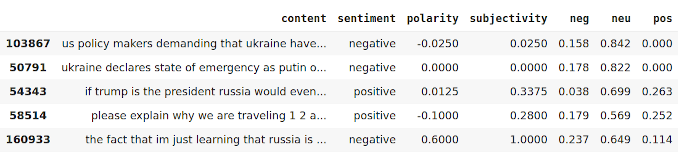
Now if we want to see the results of the above operation, then we can use the following code snippet.

Python3

tweets[["content", "sentiment", "polarity",
        "subjectivity", "neg", "neu", "pos"]].head(5)

Output:

Now to calculate the total percentage of Positive, Negative, and Neutral tweets we will use the following code snippet. 

Python3

total_pos = len(tweets.loc[tweets['sentiment'] == "positive"])
total_neg = len(tweets.loc[tweets['sentiment'] == "negative"])
total_neu = len(tweets.loc[tweets['sentiment'] == "neutral"])
total_tweets = len(tweets)
print("Total Positive Tweets % : {:.2f}"
      .format((total_pos/total_tweets)*100))
print("Total Negative Tweets % : {:.2f}"
      .format((total_neg/total_tweets)*100))
print("Total Neutral Tweets % : {:.2f}"
      .format((total_neu/total_tweets)*100))

Output:

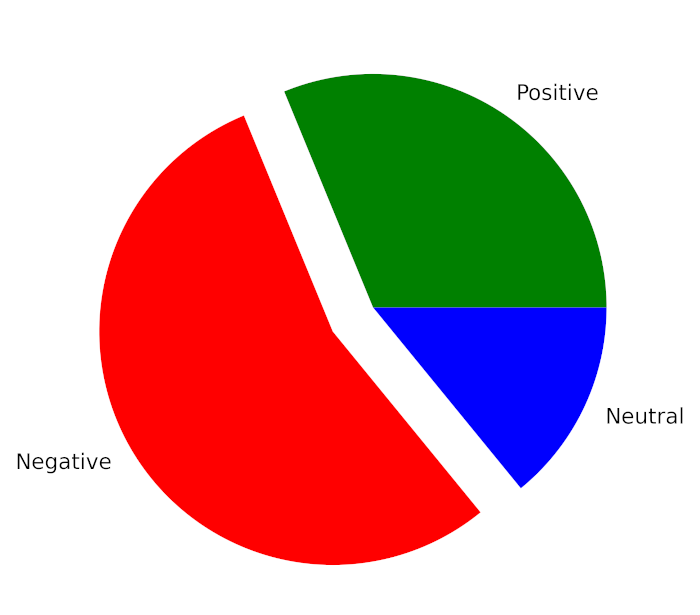
Total Positive Tweets % : 31.24
Total Negative Tweets % : 54.97
Total Neutral Tweets % : 13.79

If we want to display this result using a Pie Chart, then we can do that with the help of the below code snippet –

Python3

mylabels = ["Positive", "Negative", "Neutral"]
mycolors = ["Green", "Red", "Blue"]

plt.figure(figsize=(8, 5),
           dpi=600)  # Push new figure on stack
myexplode = [0, 0.2, 0]
plt.pie([total_pos, total_neg, total_neu], colors=mycolors,
        labels=mylabels, explode=myexplode)
plt.show()

Output:

Now, If we want to see the sentiments over 65 days, then we can do that with the help of the below code snippet.

Python3

pos_list = []
neg_list = []
neu_list = []
for i in tweets["date"].unique():
    temp = tweets[tweets["date"] == i]
    positive_temp = temp[temp["sentiment"] == "positive"]
    negative_temp = temp[temp["sentiment"] == "negative"]
    neutral_temp = temp[temp["sentiment"] == "neutral"]
    pos_list.append(((positive_temp.shape[0]/temp.shape[0])*100, i))
    neg_list.append(((negative_temp.shape[0]/temp.shape[0])*100, i))
    neu_list.append(((neutral_temp.shape[0]/temp.shape[0])*100, i))

neu_list = sorted(neu_list, key=lambda x: x[1])
pos_list = sorted(pos_list, key=lambda x: x[1])
neg_list = sorted(neg_list, key=lambda x: x[1])

x_cord_neg = []
y_cord_neg = []

x_cord_pos = []
y_cord_pos = []

x_cord_neu = []
y_cord_neu = []

for i in neg_list:
    x_cord_neg.append(i[0])
    y_cord_neg.append(i[1])


for i in pos_list:
    x_cord_pos.append(i[0])
    y_cord_pos.append(i[1])

for i in neu_list:
    x_cord_neu.append(i[0])
    y_cord_neu.append(i[1])


plt.figure(figsize=(16, 9),
           dpi=600)  # Push new figure on stack
plt.plot(y_cord_neg, x_cord_neg, label="negative", 
         color="red")
plt.plot(y_cord_pos, x_cord_pos, label="positive", 
         color="green")
plt.plot(y_cord_neu, x_cord_neu, label="neutral", 
         color="blue")
plt.xticks(np.arange(0, len(tweets["date"].unique()) + 1, 5))
plt.xticks(rotation=90)
plt.grid(axis='x')

plt.legend()

Output:

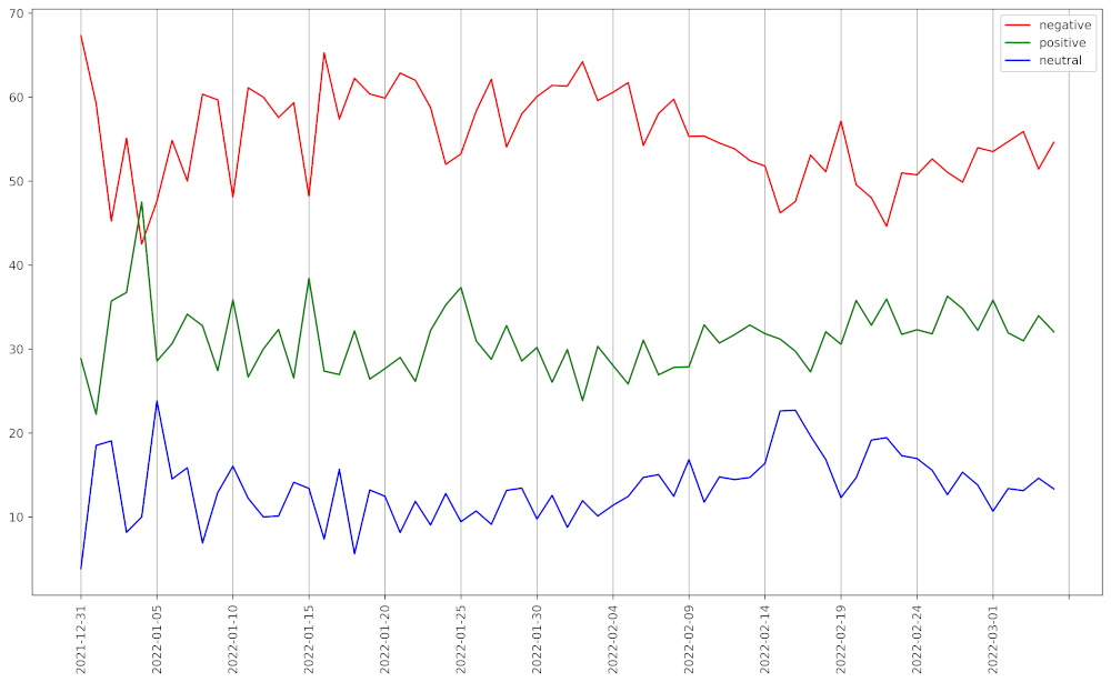
Sentiments of tweets in a graphical representation

Word Popularity using N-gram

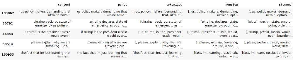
We have used the feature extraction module of Scikit-Learn to find out the most popular words and a group of adjacent words. Here we get a Bag of Word model after tokenizing, removing the stop words, and stemming on previously cleaned texts. Below is the code snippet for the same –

Python3

# make a copy of tweets named tw_list
tw_list = tweets['content']

# Removing Punctuation
def remove_punct(text):
    text = "".join([char for char in text if
                    char not in string.punctuation])
    text = re.sub('[0-9]+', '', text)
    return text


tw_list['punct'] = tw_list['content'].apply(
  lambda x: remove_punct(x))

# Applying tokenization
def tokenization(text):
    text = re.split('\W+', text)
    return text


tw_list['tokenized'] = tw_list['punct'].apply(
    lambda x: tokenization(x.lower()))

# Removing stopwords
stopword = nltk.corpus.stopwords.words('english')

def remove_stopwords(text):
    text = [word for word in text if
            word not in stopword]
    return text

tw_list['nonstop'] = tw_list['tokenized'].apply(
  lambda x: remove_stopwords(x))

# Applying Stemmer
ps = nltk.PorterStemmer()

def stemming(text):
    text = [ps.stem(word) for word in text]
    return text

tw_list['stemmed'] = tw_list['nonstop'].apply(
  lambda x: stemming(x))

tw_list.head()

# This code is modified by Susobhan Akhuli

Output:

To find out the most used words from it we need a Bag of Word first. Bag of Word is a matrix where each row represents a specific text, and each column represents a word in the vocabulary. Then a vector with the sum of each word occurrence in all texts is generated. In other words, the elements for each column of the Bag of Words matrix are added. At last, the list with the word and their occurrence count is sorted. Below is the code snippet –

Python3

# Applying Countvectorizer
countVectorizer = CountVectorizer(analyzer=clean_text)
countVector = countVectorizer.fit_transform(tw_list['content'])
count_vect_df = pd.DataFrame(
    countVector.toarray(), 
  columns=countVectorizer.get_feature_names())
count_vect_df.head()

# Most Used Words
count = pd.DataFrame(count_vect_df.sum())
countdf = count.sort_values(0, 
                            ascending=False).head(20)
countdf[1:11]

Output:

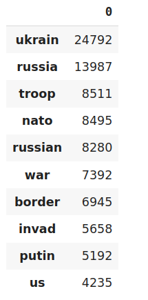
Most used words

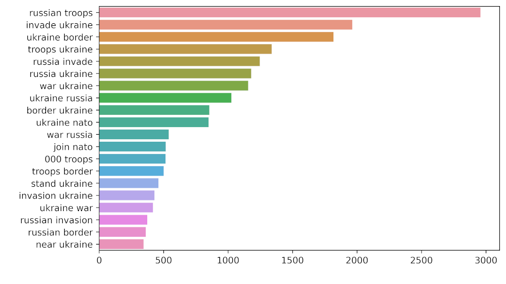
Now to find out the group of adjacent words we will take the help of Unigram and Bigram. Below is the code snippet for the same:

Python3

# Function to ngram
def get_top_n_gram(corpus, ngram_range, n=None):
    vec = CountVectorizer(ngram_range=ngram_range,
                          stop_words='english').fit(corpus)
    bag_of_words = vec.transform(corpus)
    sum_words = bag_of_words.sum(axis=0)
    words_freq = [(word, sum_words[0, idx])
                  for word, idx in vec.vocabulary_.items()]
    words_freq = sorted(words_freq, key=lambda x: x[1], reverse=True)
    return words_freq[:n]

# n2_bigram
n2_bigrams = get_top_n_gram(tw_list['content'], (2, 2), 20)
plt.figure(figsize=(8, 5),
           dpi=600)  # Push new figure on stack

sns_plot = sns.barplot(x=1, y=0, data=pd.DataFrame(n2_bigrams))
plt.savefig('bigram.jpg')  # Save that figure

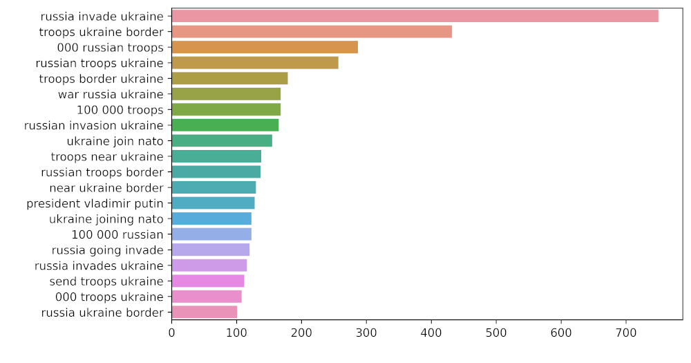
# n3_trigram
n3_trigrams = get_top_n_gram(tw_list['content'], (3, 3), 20)

plt.figure(figsize=(8, 5),
           dpi=600)  # Push new figure on stack

sns_plot = sns.barplot(x=1, y=0, data=pd.DataFrame(n3_trigrams))
plt.savefig('trigram.jpg')  # Save that figure

Output:

Bigram Representation

Trigram Representation