Fine-tuning BERT model for Sentiment Analysis
Last Updated :
02 Mar, 2022
Google created a transformer-based machine learning approach for natural language processing pre-training called Bidirectional Encoder Representations from Transformers. It has a huge number of parameters, hence training it on a small dataset would lead to overfitting. This is why we use a pre-trained BERT model that has been trained on a huge dataset. Using the pre-trained model and try to “tune” it for the current dataset, i.e. transferring the learning, from that huge dataset to our dataset, so that we can “tune” BERT from that point onwards.
In this article, we will fine-tune the BERT by adding a few neural network layers on our own and freezing the actual layers of BERT architecture. The problem statement that we are taking here would be of classifying sentences into POSITIVE and NEGATIVE by using fine-tuned BERT model.
Preparing the dataset
Link for the dataset.
The sentence column has text and the label column has the sentiment of the text – 0 for negative and 1 for positive. We first load the dataset followed by, some preprocessing before tuning the model.
Loading dataset
Python
import pandas as pd
import numpy as np
df = pd.read_csv('/content/data.csv')
|
Split dataset:
After loading the data, split the data into train, validation ad test data. We are taking the 70:15:15 ratio for this division. The inbuilt function of sklearn is being used below to split the data. We use stratified attributes to ensure that the proportion of the categories remains the same after splitting the data.
Python
from sklearn.model_selection import train_test_split
train_text, temp_text, train_labels, temp_labels = train_test_split(df['sentence'], df['label'],
random_state = 2021,
test_size = 0.3,
stratify = df['label'])
val_text, test_text, val_labels, test_labels = train_test_split(temp_text, temp_labels,
random_state = 2021,
test_size = 0.5,
stratify = temp_labels)
|
Load pre-trained BERT model and tokenizer
Next, we proceed with loading the pre-trained BERT model and tokenizer. We would use the tokenizer to convert the text into a format(which has input ids, attention masks) that can be sent to the model.
Python
bert = AutoModel.from_pretrained('bert-base-uncased')
tokenizer = BertTokenizerFast.from_pretrained('bert-base-uncased')
|
Deciding the padding length
If we take the padding length as the maximum length of text found in the training texts, it might leave the training data sparse. Taking the least length would in turn lead to loss of information. Hence, we would plot the graph and see the “average” length and set it as the padding length to trade-off between the two extremes.
Python
train_lens = [len(i.split()) for i in train_text]
plt.hist(train_lens)
|
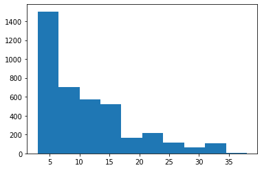
From the graph above, we take 17 as the padding length.
Tokenizing the data
Tokenize the data and encode sequences using the BERT tokenizer.
Python
tokens_train = tokenizer.batch_encode_plus(
train_text.tolist(),
max_length = pad_len,
pad_to_max_length = True,
truncation = True
)
tokens_val = tokenizer.batch_encode_plus(
val_text.tolist(),
max_length = pad_len,
pad_to_max_length = True,
truncation = True
)
tokens_test = tokenizer.batch_encode_plus(
test_text.tolist(),
max_length = pad_len,
pad_to_max_length = True,
truncation = True
)
train_seq = torch.tensor(tokens_train['input_ids'])
train_mask = torch.tensor(tokens_train['attention_mask'])
train_y = torch.tensor(train_labels.tolist())
val_seq = torch.tensor(tokens_val['input_ids'])
val_mask = torch.tensor(tokens_val['attention_mask'])
val_y = torch.tensor(val_labels.tolist())
test_seq = torch.tensor(tokens_test['input_ids'])
test_mask = torch.tensor(tokens_test['attention_mask'])
test_y = torch.tensor(test_labels.tolist())
|
Defining the model
We first freeze the BERT pre-trained model, and then add layers as shown in the following code snippets:
Python
for param in bert.parameters():
param.requires_grad = False
class BERT_architecture(nn.Module):
def __init__(self, bert):
super(BERT_architecture, self).__init__()
self.bert = bert
self.dropout = nn.Dropout(0.2)
self.relu = nn.ReLU()
self.fc1 = nn.Linear(768,512)
self.fc2 = nn.Linear(512,2)
self.softmax = nn.LogSoftmax(dim=1)
def forward(self, sent_id, mask):
_, cls_hs = self.bert(sent_id, attention_mask=mask, return_dict=False)
x = self.fc1(cls_hs)
x = self.relu(x)
x = self.dropout(x)
x = self.fc2(x)
x = self.softmax(x)
return x
|
Also, add an optimizer to enhance the performance:
Python
optimizer = AdamW(model.parameters(),lr = 1e-5)
|
Then compute class weights, and send them as parameters while defining loss function to ensure imbalance in the dataset is handled well while computing the loss.
Training the model
After defining the model, define a function to train the model (fine-tune, in this case):
Python
def train():
model.train()
total_loss, total_accuracy = 0, 0
total_preds=[]
for step,batch in enumerate(train_dataloader):
if step % 50 == 0 and not step == 0:
print(' Batch {:>5,} of {:>5,}.'.format(step, len(train_dataloader)))
batch = [r.to(device) for r in batch]
sent_id, mask, labels = batch
model.zero_grad()
preds = model(sent_id, mask)
loss = cross_entropy(preds, labels)
total_loss = total_loss + loss.item()
loss.backward()
torch.nn.utils.clip_grad_norm_(model.parameters(), 1.0)
optimizer.step()
preds=preds.detach().cpu().numpy()
total_preds.append(preds)
avg_loss = total_loss / len(train_dataloader)
total_preds = np.concatenate(total_preds, axis=0)
return avg_loss, total_preds
|
Now, define another function that would evaluate the model on validation data.
Python
print "GFG"
def evaluate():
print("\nEvaluating...")
model.eval()
total_loss, total_accuracy = 0, 0
total_preds = []
for step,batch in enumerate(val_dataloader):
if step % 50 == 0 and not step == 0:
print(' Batch {:>5,} of {:>5,}.'.format(step, len(val_dataloader)))
batch = [t.to(device) for t in batch]
sent_id, mask, labels = batch
with torch.no_grad():
preds = model(sent_id, mask)
loss = cross_entropy(preds,labels)
total_loss = total_loss + loss.item()
preds = preds.detach().cpu().numpy()
total_preds.append(preds)
avg_loss = total_loss / len(val_dataloader)
total_preds = np.concatenate(total_preds, axis=0)
return avg_loss, total_preds
|
Test the data
After fine-tuning the model, test it on the test dataset. Print a classification report to get a better picture of the model’s performance.
Python
with torch.no_grad():
preds = model(test_seq.to(device), test_mask.to(device))
preds = preds.detach().cpu().numpy()
from sklearn.metrics import classification_report
pred = np.argmax(preds, axis = 1)
print(classification_report(test_y, pred))
|
After testing, we would get the results as follows:
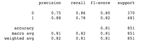
Classification report
Link to the full code.
References:
- https://huggingface.co/docs/transformers/model_doc/bert
- https://huggingface.co/docs/transformers/index
- https://huggingface.co/docs/transformers/custom_datasets
Like Article
Suggest improvement
Share your thoughts in the comments
Please Login to comment...