Stratified Boxplot in R Programming
Last Updated :
11 Oct, 2020
A boxplot is a graphical representation of groups of numerical data through their quartiles. Box plots are non-parametric that they display variation in samples of a statistical population without making any assumptions of the underlying statistical distribution. The spacings between the different parts of the box in a boxplot indicate the degree of dispersion and skewness in the data and show outliers. Boxplot can be drawn either vertically or horizontally. Boxplot got their name from the box in the middle. Stratified boxplots are used to examine the relationship between a categorical and a numeric variable, between strata or groups defined by a third categorical variable. Stratified Boxplots are useful when it comes to comparing categorical variables.
Implementation in R
In R programming stratified boxplot can be formed using the boxplot() function of the R Graphics Package.
Syntax:
boxplot(formula, data = NULL, …, subset, na.action = NULL, xlab = mklab(y_var = horizontal),
ylab = mklab(y_var =!horizontal), add = FALSE, ann = !add, horizontal = FALSE, drop = FALSE,
sep = “.”, lex.order = FALSE)
boxplot(x, …, range = 1.5, width = NULL, varwidth = FALSE, notch = FALSE, outline = TRUE, names, plot = TRUE,
border = par(“fg”), col = NULL, log = “”, pars = list(boxwex = 0.8, staplewex = 0.5, outwex = 0.5),
ann = !add, horizontal = FALSE, add = FALSE, at = NULL)
|
Parameter
|
Description
|
| formula |
a formula. |
| data |
a data.frame/list from which the variables in the formula should be taken. |
| subset |
an optional vector specifying a subset of observations to be used for plotting. |
| na.action |
a function which indicates what should happen when the data contain NAs. |
| xlab,ylab |
x- and y-axis annotation. Can be suppressed by ann=FALSE. |
| add |
logical, if true add boxplot to the current plot. |
| ann |
logical indicating if axes should be annotated (by xlab and ylab). |
| horizontal |
logical indicating if the boxplots should be horizontal; default FALSE means vertical boxes. |
| x |
for specifying data from which the boxplots are to be produced.
Either a numeric vector or a single list containing such vectors.
|
| range |
this determines how far the plot whiskers extend out from the box. |
| width |
a vector giving the relative widths of the boxes making up the plot. |
| varwidth |
if varwidth is TRUE, the boxes are drawn with widths proportional to
the square-roots of the number of observations in the groups.
|
| notch |
if the notch is TRUE, a notch is drawn in each side of the boxes. |
| outline |
if the outline is not true, the outliers are not drawn. |
| names |
group labels that will be printed under each boxplot. |
| boxwex |
a scale factor to be applied to all boxes. |
| staplewex |
staple line width expansion, proportional to box width. |
| outwex |
outlier line width expansion, proportional to box width. |
| plot |
if TRUE (the default) then a boxplot is produced. Else the summaries
which the boxplots are based on are returned.
|
| border |
an optional vector of colors for the outlines of the boxplots. |
| cols |
if col is non-null it is assumed to contain colors to be used to color
the bodies of the box plots.
|
| logs |
character indicating if x or y or both coordinates should be plotted in log scale. |
| pars |
a list of (potentially many) more graphical parameters. |
| at |
numeric vector giving the locations where the boxplots should be drawn,
particularly when add = TRUE.
|
| … |
for the formula method, named arguments to be passed to the default method. |
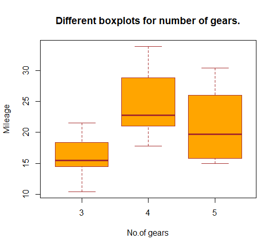
Example 1:
To plot the stratified boxplot use mtcars datasets of the datasets library in R. mtcars datasets contains data from the Motor Trend Car Road Tests. Here let’s plot the mileage(miles/gallons in this case) of different cars to the number of gears they have.
R
library(datasets)
cars <- data.frame(mtcars)
boxplot(mpg~gear, data = mtcars,
main = "Different boxplots for number of gears.",
xlab = "No.of gears",
ylab = "Mileage",
col = "orange",
border = "brown"
)
|
Example 2:
The dataset we are working with here is the LungCapData dataset which contains data on lung capacities of smokers and non-smokers of different age groups. The structure of the datasets has 6 variables each signifying lung capacity, age, height, smoke(‘yes’ for a smoker and ‘no’ for a non-smoker), gender(male/female), and Caesarean(yes/no) of a person. We will divide the ages into groups and then try to plot stratified boxplots for the lung capacity of smokers vs non-smokers with age strata. Please download the CSV file here.
R
LungCapData <- read.csv("LungCapData.csv", header = T)
LungCapData <- data.frame(LungCapData)
attach(LungCapData)
AgeGroups <- cut(LungCapData$Age,
breaks = c(0, 13, 15, 17, 25),
labels = c("<13", "14/15", "16/17", ">=18"))
head(LungCapData)
boxplot(LungCapData$LungCap~LungCapData$Smoke,
ylab = "Capacity",
main = "Lung Capacity of Smokers Vs Non-Smokers",
las = 1)
boxplot(LungCapData$LungCap[LungCapData$Age>=18]~LungCapData$Smoke[LungCapData$Age>=18],
ylab = "Capacity",
main = "Lung Capacity of Smokers Vs Non-Smokers",
las = 1)
boxplot(LungCapData$LungCap~LungCapData$Smoke*AgeGroups,
ylab = "Capacity", xlab = "",
main = "Lung Capacity of Smokers Vs Non-Smokers",
col = c(4, 2), las = 2)
|
Output:
# Boxplot 1
Boxplot 1 plots the lung capacity of smokers and non-smokers, where no symbolize non-smokers, and yes symbolizes smokers.
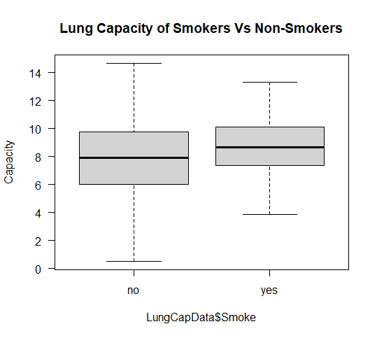
By analyzing the above-shown boxplot we can clearly say the lung capacity of non-smokers is lower as compared to that of smokers on an average.
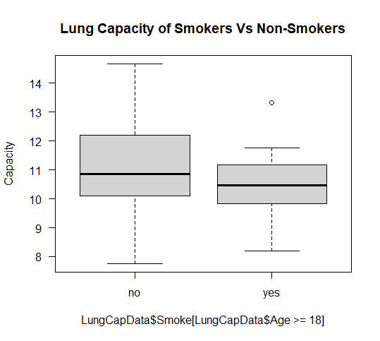
# Boxplot 2
Boxplot 2 plots the lung capacity of smokers and non-smokers of age group greater or equal to 18, where no symbolizes non-smokers and yes symbolizes smokers.
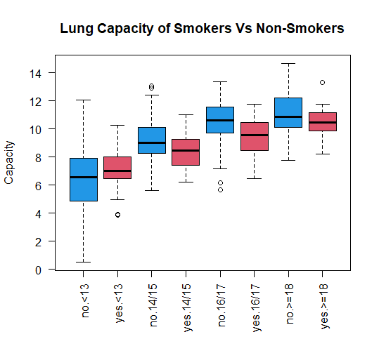
# Boxplot 3
Boxplot 3 plots the lung capacity of smokers and non-smokers of the different age groups in the dataset where blue-colored boxplots are for non-smokers and red is for smokers.
Share your thoughts in the comments
Please Login to comment...