Stacked RNNs in NLP
Last Updated :
09 Oct, 2023
Stacked RNNs refer to a special kind of RNNs that have multiple recurrent layers on top of one layer. Stacked RNNs are also called Deep RNNs for that reason. In this article, we will load the IMDB dataset and make multiple layers of SimpleRNN (stacked SimpleRNN) as an example of Stacked RNN.
What is RNN?
RNN or Recurrent Neural Network, belongs to the Neural Network family which is commonly used for Natural Language Processing (NLP) tasks. They specialize in handling any sequential data (be it video, text or time series as well). This is because of the presence of a Hidden state inside an RNN layer. The hidden state is responsible for memorizing the information from the previous timestep and using that for further adjustment of weights in Training a model.
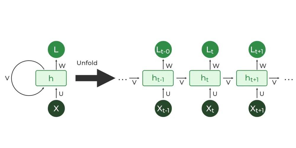
RNN architecture
What are Stacked RNNs
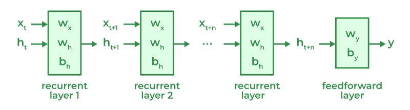
A single-layered RNN model has only a hidden layer which is liable to process sequential data. But Stacked RNN is a special kind of model that has multiple RNN layers one on each layer. This creates a ‘Stack’. Each layer of this stack processes the input sequence.
- When an Input is passed to Layer 1:
- The input (
 ) passes through the RNN layer 1. There, the hidden state gets updated as:

where = present Hidden state
 = previous hidden state
 = input to the RNN layer
 = weights associated with the input
 = weights associated with the hidden layer
 = bias associated with RNN layer
 = activation function
- What happens in the hidden state is that, using the information or knowledge it retained in the previous time step, the hidden state updates itself.
- The present hidden state is used in getting the output of the hidden layer, using an appropriate activation function.
 where,
 - W = Weights assigned to the layer
 = hidden state
 = bias associated with output layer
- For the second layer, the output of first RNN layer is fed into it, which goes through the same process again.

Stacked RNN architecture
This feature of Stacked RNNs enables to capture of both short-term and long-term patterns. For that reason, Stacked RNNs can learn and remember information patterns in longer sequences and at the same it can analyze their current state’s information with just learned previous state’s information. The more layers you add to your model, the stacked network will able to capture more complex patterns present in the sequential data. If your data is nested and has different types of complex patterns then Stacked RNNs will be a better model as its each layer can learn different abstractions present in your data.
Understanding Stacked RNN with code implementation
First we will implement the Stacked RNN as code implementation where we will output the predicted value using the model’s method.
Python3
import numpy as np
from keras.models import Sequential
from keras.layers import SimpleRNN, Dense
hidden_units = 2
input_shape = (3, 1)
input_layer = Input(shape=input_shape)
rnn_layer1 = SimpleRNN(hidden_units,return_sequences=True)(input_layer)
rnn_layer2 = SimpleRNN(hidden_units)(rnn_layer1)
output_layer = Dense(1, activation='sigmoid')(rnn_layer2)
model = Model(inputs=input_layer, outputs=output_layer)
model.compile(optimizer='adam', loss='binary_crossentropy')
model.summary()
x = np.array([1, 2, 3])
x_input = np.reshape(x, (1, 3, 1))
y_pred_model = model.predict(x_input)
print("Prediction from the neural network: \n", y_pred_model)
|
Output:
1/1 [==============================] - 0s 344ms/step
Prediction from the neural network:
 [[0.8465775]]
Now we will explore the mathematical concept behind the working of the stacked RNN
After the initial model is trained, we will get the weights associated with each layer in the architecture.
Python3
wx = model.get_weights()[0]
wh = model.get_weights()[1]
bh = model.get_weights()[2]
wx1 = model.get_weights()[3]
wh1 = model.get_weights()[4]
bh1 = model.get_weights()[5]
wy = model.get_weights()[6]
by = model.get_weights()[7]
|
As per the equations used above, the present hidden state can be explained as a function of the activation function applied on the product of weights for input and respective inputs added to the product of weights for hidden states and hidden states with bias terms.
Weights and bias distribution in RNN layers
Python3
m = 2
h = np.zeros((m))
rnn_layer1_outputs = []
for t in range(x_input.shape[1]):
h = np.tanh(np.dot(x_input[0, t], wx) + np.dot(h, wh) + bh)
rnn_layer1_outputs.append(h)
rnn_layer1_outputs = np.array(rnn_layer1_outputs)
h30 = np.zeros(2)
h31 = np.tanh(np.dot(rnn_layer1_outputs[0], wx1) +h30 + bh1)
h32 = np.tanh(np.dot(rnn_layer1_outputs[1] , wx1) + np.dot(h31,wh1) + bh1)
h33 = np.tanh(np.dot(rnn_layer1_outputs[2] , wx1) + np.dot(h32,wh1) + bh1)
outputs = 1/(1 +np.exp(-(np.dot(h33, wy) + by)))
outputs = np.array(outputs)
print("Prediction from manual computation: \n", outputs)
|
Output:
Prediction from manual computation:
 [0.84657752]
Why we will use Stacked RNNs
Using Stacked RNNs can give us several benefits which are listed below–>
- Modeling Complex Dependencies: Stacked RNNs are well-aware of modelling complex and nested dependencies in sequential data. For that reason, Stacked RNNs can automatically capture information at different time-stamps or levels of abstraction which are need to be learned.
- Improved Representation: A sequential data contains different types or levels of features. Stacked RNNs are capable to capture these features level wise which means its initial or lower level layers capture lower level or basic features whereas its higher layers capture high-leveled features. This leads to improved model performance and high-end feature engineering.
- Long-Term Dependencies: For many real-world applications, it is essential to remember the earlier parts of a sequence to make accurate predictions or decisions(for example Stock market price prediction, sentiment analysis etc.). Stacked RNNs can effectively remember the past learned sequences to handle long-term dependencies by passing information from one layer to the next layer of its stack.
- Reducing Vanishing Gradient Problem: While training deep network models, vanishing gradient problem is very common issue can be faced most of the time. This occurs because when the gradients are updating step by step it becomes smell then smaller and then may be vanished. It leads to errors in prediction and degrades model performance badly. But Stacked RNNs have gating mechanism which allow smooth flow of gradients through the network and monitors training states to stop the gradients become vanished.
Architecture of Stacked RNNs
The architecture of Stacked RNNs can be divided into three parts which are discussed below–>
- Number of Layers: The number of layers is a hyperparameter of stacked RNN model that can be tuned based on the complexity of the task. More number of stacks can capture more intricate patterns. But be cautious during selecting number of layers because more layers may require more training data and longer training times. If your data sequence is short then don’t use more that 2-3 layers because un-necessarily extra training time may lead to make your model un-optimized.
- Dropout and Regularization: Stacked RNNs are not proofed from model overfitting problem. To prevent this problem, Stacked RNNs have dropout and regularization techniques which can be applied between RNN layers. This helps to improve the generalization ability of the model.
- Layer Types: Stacked RNNs generally has three types of layer options which are vanilla RNNs, LSTMs and GRUs. Most popular layers are LSTM and GRU as they can handle long-term dependencies and mitigate the vanishing gradient problem.
Step-by-step implementation and visualization
Importing dependencies
At first, we will import all necessary Python libraries like NumPy, TensorFlow , Matplotlib etc.
Python3
import numpy as np
import tensorflow as tf
from tensorflow.keras.models import Sequential
from tensorflow.keras.layers import SimpleRNN, Embedding, Dense
from tensorflow.keras.datasets import imdb
from tensorflow.keras.preprocessing import sequence
import matplotlib.pyplot as plt
|
Dataset Loading
Now we will load IMDB dataset and define our desired maximum number of features (words) to consider in the vocabulary, maximum length of movie reviews (sequences) and the batch size for model training.
Python3
max_features = 10000
maxlen = 80
batch_size = 32
(x_train, y_train), (x_test, y_test) = imdb.load_data(num_words=max_features)
x_train = sequence.pad_sequences(x_train, maxlen=maxlen)
x_test = sequence.pad_sequences(x_test, maxlen=maxlen)
|
Building the Stacked RNN model and compile
Now we will build a two layered stacked RNN model. Each RNN layer takes in units (here, we have taken it as 64) which is a positive integer and gives the output dimensionality of the layer. Since, we have not provided any activation function, it will take the default “Tanh” activation.
Python3
model = Sequential()
model.add(Embedding(max_features, 128, input_length=maxlen))
model.add(SimpleRNN(64, return_sequences=True))
model.add(SimpleRNN(64))
model.add(Dense(1, activation='sigmoid'))
tf.keras.utils.plot_model(model, show_shapes = True,
to_file='stacked_rnn_model.png',
show_dtype = True,
show_layer_activations = True)
|
Output:

Model summary
(Note: Here we are using Return_sequences = True, because this model is used for text generation. This is widely used in Sequence to sequence modelling.)
Compiling the model and fitting
Here, we are optimizing our model with Adam optimizer, and for our metrics we are using accuracy. Since, this is a language model, we are choosing the loss function as Binary cross entropy. Binary Cross entropy is a useful loss function when doing a classification between two variables.
Python3
model.compile(loss='binary_crossentropy',
optimizer='adam',
metrics=['accuracy'])
history = model.fit(x_train,
y_train,
batch_size=batch_size,
epochs=5,
validation_data=(x_test, y_test))
|
Output:
Epoch 1/5
782/782 [================] - 71s 86ms/step - loss: 0.5839 - accuracy: 0.6674 - val_loss: 0.4865 - val_accuracy: 0.7664
Epoch 2/5
782/782 [================] - 58s 74ms/step - loss: 0.3997 - accuracy: 0.8253 - val_loss: 0.4886 - val_accuracy: 0.7672
Epoch 3/5
782/782 [================] - 58s 74ms/step - loss: 0.2759 - accuracy: 0.8881 - val_loss: 0.5004 - val_accuracy: 0.8018
Epoch 4/5
782/782 [================] - 58s 74ms/step - loss: 0.1842 - accuracy: 0.9313 - val_loss: 0.5710 - val_accuracy: 0.7909
Epoch 5/5
782/782 [================] - 57s 73ms/step - loss: 0.1079 - accuracy: 0.9611 - val_loss: 0.7576 - val_accuracy: 0.7653
Visualization of results
Now we will plot the metrics like Accuracy and loss (Binary Cross Entropy) with epochs.
Python3
plt.figure(figsize=(12, 6))
plt.plot(history.history['loss'], label='Loss (MSE)')
plt.plot(history.history['val_loss'], label='Validation Loss (MSE)')
plt.plot(history.history['accuracy'], label='accuracy')
plt.plot(history.history['val_accuracy'], label='Validation accuracy')
plt.xlabel('Epochs')
plt.ylabel('Metrics')
plt.xticks(range(1, len(history.history['loss']) + 1))
plt.legend()
plt.title('Training Metrics Over Epochs')
plt.grid(False)
plt.savefig('Plots_of_stacked_rnn.png')
plt.show()
|
Output:
.jpg)
Plotting the metrics
Model evaluation on test data
Now we evaluate out stacked LSTM model on test set.
Python3
loss, accuracy= model.evaluate(x_test, y_test)
print("Test Loss:", loss)
print("Test Accuracy:", accuracy)
|
Output:
782/782 [==============================] - 12s 15ms/step - loss: 0.7576 - accuracy: 0.7653
Test Loss: 0.7575814723968506
Test Accuracy: 0.7653200030326843
Conclusion
So, from results we can say that out Stacked LSTM model is very efficient as it achieved 83.16% accuracy and Loss(MSE) and MAE both error functions is very low which shows the dependability a stacked RNN structure shows.
Share your thoughts in the comments
Please Login to comment...