Single Slit Diffraction Pattern using Python
Last Updated :
25 Sep, 2023
This article discusses a basic idea to create/simulate the diffraction pattern of a single slit on a screen placed in front of it at a distance for a monochromatic light. We don’t use any simulation library here and the article is not meant for professional-level simulation. Instead, the intention is to show an example to the reader about how to use programming skills to simulate real-world things. Moreover, this can also serve as a moderate-level Python project. Before we proceed, you need to know that this article assumes basic familiarity with Python programming language and little familiarity with its NumPy and Matplotlib packages
What is Diffraction?
Diffraction is the phenomenon of bending of light at the edges of obstacles and is caused by the wave nature of light. This gives rise to lots of commonly known concepts in optics. One such concept is an experiment to get the diffraction pattern of a single slit on a screen placed in front of it at some distance. We are going to roughly simulate this very experiment and obtain the image formed on the screen. We will take a monochromatic light source (i.e., light containing only one wavelength) to keep things simple. The superposition principle will be used to obtain the intensity/amplitude of light at different points on the screen.
If you are completely unfamiliar with this concept and finding the terms uncomfortable, you can refer to the ‘Further Resources’ section of this article to get basic familiarity with this concept and continue from here after that.
Algorithm
In this simulation, we place the slit at the origin of the coordinate system (i.e., the center of the slit is at (0,0,0)) and the screen is placed at some perpendicular distance (Z) towards the positive z-axis parallel to the slit. The light is coming from the negative z direction towards the positive z direction as shown in this figure
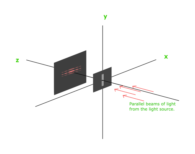
Theoretical setup for simulating single slit diffraction pattern on a computer.
The result of our simulation will be a rough image of the pattern formed on the screen.
As per the theory of this experiment, all the beams leaving the slit and incident on the screen are in the same phase (i.e., coherent). At each point on the screen the intensity/amplitude of light is given by the superposition of the intensities (with their phase) due to beam coming from each point on the slit. So, the steps to implement the idea are as follows –
- Step 1: Divide the screen into M rows and N columns (thus obtaining MxN sample points on the screen).
- Step 2: Divide the slit into P rows and Q columns (thus obtaining PxQ sample points on slit) similar step 1.
- Step 3: Create a MxN array (A) representing the intensity/amplitude of light at the sample-points on the screen.
- Step 4: For each sample point on the screen, calculate the intensity of light at the point and store the absolute value at the corresponding location in the intensity array A.
- Step 5: Create a heatmap of the array A. (Heatmap is a graph representing data in the form of a map or diagram in which data values are represented as colors)
Here are more details for the step-4 given above:
Intensity at a point on the screen = absolute value of (sum of all the intensities at the point with proper sign (+/-) due to each point on the slit).
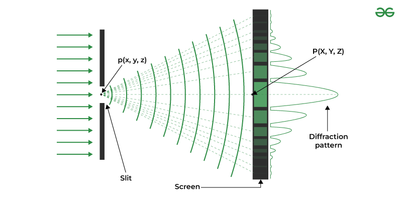
If p = (x, y, z) is a point on the slit and P = (X, Y, Z) is a point on the screen, then, the intensity at P due to p can be given by –

where, a is the amplitude, the square root expression is the distance between the points p and P (distance formula), lambda is the wavelength of the light and phi is the initial phase angle. For our simulation, we assume all the waves to have zero phase angle and z = 0 always since the slit is at z = 0. So, the formula for our case becomes –

Also, we choose to simulate for the wavelength ( ) = 600nm (approximately corresponding to red light).
Complexity of the Algorithm
The asymptotic time complexity is O(MxNxn), and space complexity is O(MxN) for the above algorithm. Where n represents the number of sample points taken on the slit.
Code Implementation
Required Installation
Before we begin to code, we need to have python-3 interpreter installed on our system along with NumPy and Matplotlib packages. If you prefer your own setup or have Linux, then great! Otherwise on windows, you can install the packages by running the following commands on the command-prompt/terminal once the python interpreter is installed –
py -m pip install numpy
py -m pip install matplotlib
Implement of the Algorithm in Python
There can be multiple ways to implement the above algorithm in python. This code uses NumPy for arrays and their manipulation and Matplotlib for creating the heatmap. The rest of the details are as per the details stated in the ‘Algorithm’ section. Moreover, detailed description of the steps are provided in comments inside the code.
Python3
import numpy as np
import matplotlib.pyplot as plt
import matplotlib.colors
D = 5
slitWidth = 0.0001
slitHeight = 0.005
a = 1
w = 0.0000006
x1 = -0.25
x2 = 0.25
y1 = -0.025
y2 = 0.025
lres = 5000
m, n = int((x2-x1)*lres), int((y2-y1)*lres)
X = np.linspace(x1, x2, n)
Y = np.linspace(y1, y2, m)
X, Y = np.meshgrid(X, Y)
Z = np.ones((m, n))*D
xcoords = np.linspace(-slitWidth/2, slitWidth/2, 20)
ycoords = np.linspace(-slitHeight/2, slitHeight/2, 100)
A = np.zeros((m, n))
for i in ycoords:
for j in xcoords:
L = np.sqrt(np.square(X-np.ones((m, n))*j) +
np.square(Y-np.ones((m, n))*i) + np.square(Z))
theta = (L/w) * 2 * np.pi
A += a * np.sin(theta)
A = np.abs(A)
ax = plt.axes()
ax.set_aspect('equal')
plt.rc('text', usetex=False)
plt.title("Single Slit Diffraction Pattern Simulation\nD = {}m, slit-width = {}m, slit-height = {}m, $\lambda$ = {}m".format(D, slitWidth, slitHeight, w))
plt.xlabel("x-axis of screen (metres)")
plt.ylabel("y-axis (metres)")
graph = plt.pcolormesh(
X, Y, A, cmap=matplotlib.colors.LinearSegmentedColormap.from_list("", ['black', 'red']))
plt.colorbar(graph, orientation='horizontal')
plt.show()
|
You can set cmap = “Greys_r” to see the black and white output. It is adjusted to red here to hint that the wavelength corresponds to red-light. You can try adjusting the different parameters to see different results. You can adjust the linear resolution (lres) to high or low depending upon the performance of your system.
Output
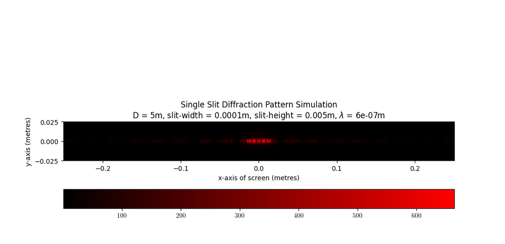
Single slit diffraction pattern generated using Python3, Matplotlib and NumPy.
Share your thoughts in the comments
Please Login to comment...