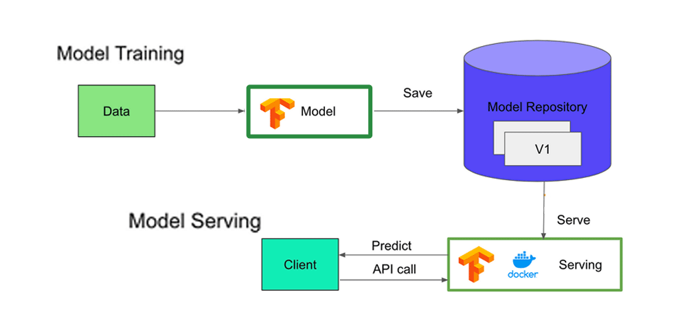
TensorFlow Serving stands as a versatile and high-performance system tailored for serving machine learning models in production settings. Its primary objective is to simplify the deployment of novel algorithms and experiments while maintaining consistent server architecture and APIs. While it seamlessly integrates with TensorFlow models, TensorFlow Serving’s adaptability also enables the service to be expanded for serving diverse model types and data beyond TensorFlow.
TensorFlow Serving
Tensorflow servable architecture consists of four components: servables, loaders, managers, and core. The explanation for the same are:
1. Servables
Servables can be considered as the core abstraction in TensorFlow Serving. Servables are the objects that are used by clients to perform the computations like inference or lookup. Servables are available in flexible size and granularity, and a single Servable may be anything from a single model to a tuple of inference models. Servables allow flexibility and future improvements such as streaming results, experimental APIs, and asynchronous modes of operation. They do not manage their own life cycles. A Servable may include:
- TensorFlow SavedModelBundle (tensorflow::Session)
- Lookup table for embedding or vocabulary lookups
Servable Versions: A TensorFlow Serving can handle one or more versions of servable over the lifetime of a single instance of the server. Versions allows multiple versions of the serverable to be loaded concurrently. They help in experimentation and gradual roll-outs.
Models: TF Serving represents the model as one or more servables and may contain one or more algorithms, lookups or embeddings. A composite model may be represented as multiple independent servables or single composite servables.
Servable Streams: These are the sequence of versions of servables sorted in ascending order.
2. Loaders
Loaders play a pivotal role in overseeing the lifecycle of a servable. They leverage the Loader API to establish a uniform infrastructure that operates independently of the underlying learning algorithms, data, or product use cases. In essence, Loaders provide a standardized set of interfaces for the loading and unloading of servables, ensuring consistent management practices.
3. Sources
Sources represent plugin modules responsible for locating and furnishing servables. A Source is often connected with zero or more SourceAdapters, and the final component in this chain is responsible for emitting the Loaders. TF Serving’s interface for Sources is designed to discover servables from diverse storage systems. Additionally, TensorFlow Serving incorporates standard reference implementations for Sources. These Sources can leverage various mechanisms such as remote procedure calls (RPC) or file system polling to access servables. One notable feature of Sources is their ability to maintain shared state across multiple servables or versions.
Aspired Versions: Aspired versions denote the collection of serviceable versions that need to be loaded and prepared. Sources convey this set of serviceable versions for a single serviceable stream at any given moment. When a Source provides a new roster of aspired versions to the Manager, it supersedes the previous roster for that particular serviceable stream. The Manager proceeds to unload any previously loaded versions that are no longer included in the new list.
4. Managers
Managers handle full life cycle of Servables including: loading, serving and unloading the Servables. Managers monitor Sources and maintain a record of all available versions. While Managers make an effort to satisfy the requests from Sources, there may be situations where they decline to load a desired version due to, for instance, insufficient resources. Additionally, Managers have the flexibility to delay the unloading of a version. For instance, they might opt to postpone unloading until a newer version has completed loading, adhering to a policy that ensures there is always at least one loaded version at any given time. TF Serving Managers provide a simple, narrow interface — GetServableHandle() — for clients to access loaded servable instances.
5. Core
TF core manages services like lifecycle and metrics using the TensorFlow Serving. It treats servables and loaders as opaque objects.
Lifecycle of a Servable
Lifecycle of a Servable is defined as:
1. Loader Creation: Initially, a Source plugin is responsible for crafting a Loader tailored to a specific version of a Servable. This Loader is equipped with all the essential metadata necessary for the subsequent loading of the Servable.
2. Aspired Version Notification: The Source employs a callback mechanism to relay information about the Aspired Version to the Manager. This signifies the version that the system should ideally have loaded and ready for use.
3. Version Policy Application: Upon receiving the Aspired Version information, the Manager enters the decision-making phase. It employs the Version Policy that has been configured to determine the most appropriate action to take next. This action can vary and might involve unloading a previously loaded version to make way for the Aspired Version or initiating the loading process for the new version.
4. Resource Allocation and Loading: If the Manager, following the guidelines of the Version Policy, decides that it is safe and feasible to proceed, it proceeds to allocate the necessary resources to the Loader. Once the required resources are allocated, the Manager instructs the Loader to commence the loading procedure for the new version.
5. Servable Access for Clients: Clients who require access to the Servable interact with the Manager. Clients have the option to either explicitly specify the desired version they wish to use or simply request the latest available version. In response, the Manager furnishes the clients with a handle or reference that enables them to access and utilize the Servable as needed.
TensorFlow Serving
Requirements
To run tensorflow servings, you need to have Ubuntu or docker. DO NOT TRY TO INSTALL APT-GET AS IT WILL NOT WORK, TRY DOCKER INSTEAD FOR YOUR OS.
On Ubuntu
On your machine, run the following command to add packages to apt repository:
!echo "deb [arch=amd64] http://storage.googleapis.com/tensorflow-serving-apt stable tensorflow-model-server tensorflow-model-server-universal" | sudo tee /etc/apt/sources.list.d/tensorflow-serving.list && \
curl https://storage.googleapis.com/tensorflow-serving-apt/tensorflow-serving.release.pub.gpg | sudo apt-key add -
Install TensorFlow Serving
$ wget 'http://storage.googleapis.com/tensorflow-serving-apt/pool/tensorflow-model-server-2.8.0/t/tensorflow-model-server/tensorflow-model-server_2.8.0_all.deb'
$ dpkg -i tensorflow-model-server_2.8.0_all.deb
$ pip3 install tensorflow-serving-api==2.8.0
Build the model
Step 1: Import the necessary libraries
Python3
import tensorflow as tf
from tensorflow import keras
import numpy as np
import matplotlib.pyplot as plt
import os
import subprocess
|
Step 2: Load the dataset
Python3
(data_train, label_train), (data_test, label_test) = keras.datasets.cifar10.load_data()
print('Train data :',data_train.shape,label_train.shape)
print('Test data :',data_test.shape,label_test.shape)
|
Output:
Train data : (50000, 32, 32, 3) (50000, 1)
Test data : (10000, 32, 32, 3) (10000, 1)
Number of classes
Python3
classes = ['aeroplane', 'automobile', 'bird', 'cat', 'deer', 'dog', 'frog', 'horse', 'ship', 'truck']
num_classes = len(classes)
num_classes
|
Output:
10
Step 3: Build the model
Python3
model = keras.models.Sequential()
model.add(keras.layers.Conv2D(32, (3, 3), activation='relu', input_shape=(32, 32, 3)))
model.add(keras.layers.MaxPooling2D((2, 2)))
model.add(keras.layers.Conv2D(64, (3, 3), activation='relu'))
model.add(keras.layers.MaxPooling2D((2, 2)))
model.add(keras.layers.Conv2D(128, (3, 3), activation='relu'))
model.add(keras.layers.Conv2D(128, (3, 3), activation='relu'))
model.add(keras.layers.MaxPooling2D((2, 2)))
model.add(keras.layers.Flatten())
model.add(keras.layers.Dense(256, activation='relu'))
model.add(keras.layers.Dense(num_classes, activation='softmax'))
model.compile(optimizer='adam',
loss=tf.keras.losses.SparseCategoricalCrossentropy(from_logits=True),
metrics=[keras.metrics.SparseCategoricalAccuracy()])
model.summary()
|
Output:
Model: "sequential"
_________________________________________________________________
 Layer (type)                Output Shape              Param #
=================================================================
 conv2d (Conv2D)             (None, 30, 30, 32)        896

 max_pooling2d (MaxPooling2D  (None, 15, 15, 32)       0
 )

 conv2d_1 (Conv2D)           (None, 13, 13, 64)        18496

 max_pooling2d_1 (MaxPooling  (None, 6, 6, 64)         0
 2D)

 conv2d_2 (Conv2D)           (None, 4, 4, 128)         73856

 conv2d_3 (Conv2D)           (None, 2, 2, 128)         147584

 max_pooling2d_2 (MaxPooling  (None, 1, 1, 128)        0
 2D)

 flatten (Flatten)           (None, 128)               0

 dense (Dense)               (None, 256)               33024

 dense_1 (Dense)             (None, 10)                2570

=================================================================
Total params: 276,426
Trainable params: 276,426
Non-trainable params: 0
_________________________________________________________________
Step 4: Train the model
Python3
epoch = 4
model.fit(data_train, label_train, epochs=epoch)
|
Output:
Epoch 1/4
1563/1563 [==============================] - 14s 8ms/step - loss: 1.6731 - sparse_categorical_accuracy: 0.4234
Epoch 2/4
1563/1563 [==============================] - 14s 9ms/step - loss: 1.2742 - sparse_categorical_accuracy: 0.5499
Epoch 3/4
1563/1563 [==============================] - 17s 11ms/step - loss: 1.1412 - sparse_categorical_accuracy: 0.5994
Epoch 4/4
1563/1563 [==============================] - 17s 11ms/step - loss: 1.0541 - sparse_categorical_accuracy: 0.6328
<keras.callbacks.History at 0x7f6f5c532920>
Step 5: Evaluate the model
Python3
loss, accuracy_ = model.evaluate(data_test, label_test)
print()
print(f"Test accuracy: {accuracy_*100}")
print(f"Test loss: {loss}")
|
Output:
313/313 [==============================] - 1s 4ms/step - loss: 1.0704 - sparse_categorical_accuracy: 0.6358

Test accuracy: 63.58000040054321
Test loss: 1.0704132318496704
Step 6: Save the model
Python3
import tempfile
import os
curr_version = 1
my_dir = tempfile.gettempdir()
path = os.path.join(my_dir, str(curr_version))
print(f'Export Path = {path}\n')
model.save(path, overwrite=True, include_optimizer=True, save_format=None, signatures=None, options=None)
print('\nSaved model:')
import glob
file_list = glob.glob(f'{path}/*')
for file in file_list:
print(file)
|
Output:
Export Path = /tmp/1
INFO:tensorflow:Assets written to: /tmp/1/assets

Saved model:
/tmp/1/fingerprint.pb
/tmp/1/saved_model.pb
/tmp/1/assets
/tmp/1/variables
/tmp/1/keras_metadata.pb
Deployment
Step 1: Check the saved model
Python3
!saved_model_cli show --dir {path} --all
|
Output:
2023-09-15 14:34:42.403572: W tensorflow/compiler/tf2tensorrt/utils/py_utils.cc:38] TF-TRT Warning: Could not find TensorRT

MetaGraphDef with tag-set: 'serve' contains the following SignatureDefs:

signature_def['__saved_model_init_op']:
  The given SavedModel SignatureDef contains the following input(s):
  The given SavedModel SignatureDef contains the following output(s):
    outputs['__saved_model_init_op'] tensor_info:
        dtype: DT_INVALID
        shape: unknown_rank
        name: NoOp
  Method name is:

signature_def['serving_default']:
  The given SavedModel SignatureDef contains the following input(s):
    inputs['conv2d_input'] tensor_info:
        dtype: DT_FLOAT
        shape: (-1, 32, 32, 3)
        name: serving_default_conv2d_input:0
  The given SavedModel SignatureDef contains the following output(s):
    outputs['dense_1'] tensor_info:
        dtype: DT_FLOAT
        shape: (-1, 10)
        name: StatefulPartitionedCall:0
  Method name is: tensorflow/serving/predict
The MetaGraph with tag set ['serve'] contains the following ops: {'AssignVariableOp', 'StringJoin', 'BiasAdd', 'StatefulPartitionedCall', 'Pack', 'MaxPool', 'SaveV2', 'VarHandleOp', 'Identity', 'Softmax', 'NoOp', 'StaticRegexFullMatch', 'Relu', 'Const', 'DisableCopyOnRead', 'MatMul', 'MergeV2Checkpoints', 'Reshape', 'Conv2D', 'Select', 'Placeholder', 'RestoreV2', 'ShardedFilename', 'ReadVariableOp'}

Concrete Functions:
  Function Name: '__call__'
    Option #1
      Callable with:
        Argument #1
          inputs: TensorSpec(shape=(None, 32, 32, 3), dtype=tf.float32, name='inputs')
        Argument #2
          DType: bool
          Value: True
        Argument #3
          DType: NoneType
          Value: None
    Option #2
      Callable with:
        Argument #1
          conv2d_input: TensorSpec(shape=(None, 32, 32, 3), dtype=tf.float32, name='conv2d_input')
        Argument #2
          DType: bool
          Value: True
        Argument #3
          DType: NoneType
          Value: None
    Option #3
      Callable with:
        Argument #1
          conv2d_input: TensorSpec(shape=(None, 32, 32, 3), dtype=tf.float32, name='conv2d_input')
        Argument #2
          DType: bool
          Value: False
        Argument #3
          DType: NoneType
          Value: None
    Option #4
      Callable with:
        Argument #1
          inputs: TensorSpec(shape=(None, 32, 32, 3), dtype=tf.float32, name='inputs')
        Argument #2
          DType: bool
          Value: False
        Argument #3
          DType: NoneType
          Value: None

  Function Name: '_default_save_signature'
    Option #1
      Callable with:
        Argument #1
          conv2d_input: TensorSpec(shape=(None, 32, 32, 3), dtype=tf.float32, name='conv2d_input')

  Function Name: 'call_and_return_all_conditional_losses'
    Option #1
      Callable with:
        Argument #1
          inputs: TensorSpec(shape=(None, 32, 32, 3), dtype=tf.float32, name='inputs')
        Argument #2
          DType: bool
          Value: True
        Argument #3
          DType: NoneType
          Value: None
    Option #2
      Callable with:
        Argument #1
          inputs: TensorSpec(shape=(None, 32, 32, 3), dtype=tf.float32, name='inputs')
        Argument #2
          DType: bool
          Value: False
        Argument #3
          DType: NoneType
          Value: None
    Option #3
      Callable with:
        Argument #1
          conv2d_input: TensorSpec(shape=(None, 32, 32, 3), dtype=tf.float32, name='conv2d_input')
        Argument #2
          DType: bool
          Value: False
        Argument #3
          DType: NoneType
          Value: None
    Option #4
      Callable with:
        Argument #1
          conv2d_input: TensorSpec(shape=(None, 32, 32, 3), dtype=tf.float32, name='conv2d_input')
        Argument #2
          DType: bool
          Value: True
        Argument #3
          DType: NoneType
          Value: None
Step 2: Define the model directory
Python3
import os
os.environ["MODEL_DIR"] = my_dir
|
Step 3: Start TensorFlow Model Server
Python3
import subprocess
command = f"nohup tensorflow_model_server --rest_api_port=8501 --model_name=CIFARModel --model_base_path='{my_dir}' > server.log 2>&1"
subprocess.Popen(command, shell=True)
|
Output:
<Popen: returncode: None args: "nohup tensorflow_model_server --rest_api_por...>
Check the server log
Output:
2023-09-15 14:34:44.080115: E external/org_tensorflow/tensorflow/core/grappler/optimizers/meta_optimizer.cc:828]
tfg_optimizer{} failed: NOT_FOUND: Op type not registered 'DisableCopyOnRead' in binary running on GFG19509-LAPTOP.
Make sure the Op and Kernel are registered in the binary running in this process. Note that if you are loading a saved graph
which used ops from tf.contrib, accessing (e.g.) `tf.contrib.resampler` should be done before importing the graph,
as contrib ops are lazily registered when the module is first accessed.
    when importing GraphDef to MLIR module in GrapplerHook
Step 4: Request to the model in TensorFlow Serving to Predict the label of test images
Plot the first 10 test images with their lables
Python3
import matplotlib.pyplot as plt
def plot_images(images, titles, rows=2, cols=5):
fig, axes = plt.subplots(rows, cols, figsize=(13, 5))
for i, ax in enumerate(axes.ravel()):
ax.imshow(images[i].reshape(32, 32, 3))
ax.axis('off')
ax.set_title(titles[i])
sample_indices = np.linspace(0,9,10,dtype=int)
sample_images = [data_test[i] for i in sample_indices]
sample_labels = [classes[label_test[i].item()] for i in sample_indices]
plot_images(sample_images, sample_labels)
plt.show()
|
Output:
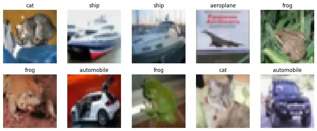
Test images with Actual label
Create JSON Object
Create JSON Object with JSON library as shown the code below. I have used official code, you may modify code for your needs accordingly.
Python3
import json
signature_name = "serving_default"
instances = data_test[0:10].tolist()
data_dict = {
"signature_name": signature_name,
"instances": instances
}
data = json.dumps(data_dict)
print(f'Data: {data[:50]} ... {data[-52:]}')
|
Output:
Data: {"signature_name": "serving_default", "instances": ... 164, 163, 204], [182, 182, 225], [186, 185, 223]]]]}
RUN Experiments
To run experiments, we need to define JSON Objects, install requests, and do some visualisation.
Install Requests
We will install the requests library. Run the following bash command:
!pip install -q requests
Run the following Python 3 code:
Python3
import requests
import json
headers = {"content-type": "application/json"}
response = requests.post(api_url, data=data, headers=headers)
if response.status_code == 200:
response_data = json.loads(response.text)
predictions = response_data['predictions']
else:
print(f"Failed to make a request. Status code: {response.status_code}")
|
Now run the following codes to check the classes of both predicted and actual label:
Python3
for prediction in predictions:
target = max(prediction)
object_ = prediction.index(target)
print(classes[object_])
|
Output:
cat
ship
ship
aeroplane
frog
frog
automobile
frog
cat
truck
You can see the output taken from the model which is around 70% accurate and matches the model accuracy.
Share your thoughts in the comments
Please Login to comment...