Python – PyTorch atan2() method

PyTorch atan2() method computes element-wise arctangent of (y/x), where y, x are the tensors with y-coordinates and x-coordinates of the points respectively. The arctangent of (y/x) is the angle between the positive x-axis and the line from (0,0) to the (x,y). So the atan2() method computes these angles. These angles are measured in radians and are in the range [-pi, pi]. These angles are computed using the help of the quadrant of the points. The quadrants can be returned using the signs of the elements of the input tensors. Mathematically it can also be termed as a 2-argument arctangent (atan2).

torch.atan2() function:

Syntax: torch.atan2(input, other, out=None)

Parameters:

• input: the first input tensor (y-coordinates).
• other: the second input tensor (x coordinates).
• out: the output tensor, a keyword argument.

Return: It returns a new tensor with element-wise arctangent of (input/other).

Example 1:

In this example, we compute element-wise 2-argument arctangent values for two input tensors, here the 2-argument arctangent is computed element-wise.

Python3

# Python 3 program to demonstrate torch.atan2() method
# importing torch
import torch

# defining first tensor (y-coordinates)
y = torch.tensor([0., 40., -137., -30.])

# defining second tensor (x-coordinates)
x = torch.tensor([120., -4., -70., 23.])

# printing the two tensors
print('Tensor y:', y)
print('Tensor x:', x)

# computing the 2-argument arc tangent
result = torch.atan2(y, x)
print('atan2(y,x):', result)

Output:

Tensor y: tensor([   0.,   40., -137.,  -30.])
Tensor x: tensor([120.,  -4., -70.,  23.])
atan2(y,x): tensor([ 0.0000,  1.6705, -2.0432, -0.9167])

Example 2:

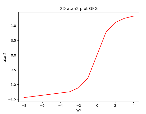
In the example below we compute element-wise 2-argument arctangent and visualize the result as a 2D plot using Matplotlib. Here, we plot a 2D graph between the “y/x” values and “atan2()”.  The “y/x” values are plotted on the x-axis and “atan2()” values on the y-axis. Notice that on increasing the value of the atan2() increases.

Python3

# Python3 program to demonstrate torch.atan2() method
%matplotlib qt

# importing required libraries
import torch
import numpy as np
import matplotlib.pyplot as plt

# defining first tensor (y-coordinates)
b = np.array([-8,-3,-2,-1,0,1,2,3,4])

# defining second tensor (x-coordinates)
a = np.array([1,1,1,1,1,1,1,1,1])
y = torch.tensor(b)
x = torch.tensor(a)
print('Tensor y:\n', y)
print('Tensor x:\n', x)

# computing the 2-argument arc tangent
result = torch.atan2(y,x)
print('atan2:\n', result)

# tensor to numpy array
result = result.numpy()

# plot the result using matplotlib
plt.plot(b/a, result, color='r', label='atan2')
plt.xlabel("y/x")
plt.ylabel("atan2")
plt.title("2D atan2 plot GFG")
plt.show()

Output:

Tensor y:

 tensor([-8, -3, -2, -1,  0,  1,  2,  3,  4], dtype=torch.int32)

Tensor x:

 tensor([1, 1, 1, 1, 1, 1, 1, 1, 1], dtype=torch.int32)

atan2:

 tensor([-1.4464, -1.2490, -1.1071, -0.7854,  0.0000,  0.7854,  1.1071,  1.2490,

         1.3258])

Example 3:

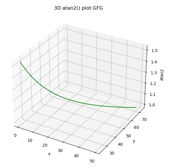
In the example below we compute element-wise 2-argument arctangent and visualize the result as a 3D plot using Matplotlib. Here, we plot a 3D graph between the “x”, “y” a,nd “atan2()”.  The “x” values are plotted on the x-axis, The “y” values are plotted on the y-axis, and the “atan2()” values are on the z-axis. Notice how the atan2() is related to the x and y.

Python3

# Python3 program to demonstrate torch.atan2() method
%matplotlib qt

# importing required libraries
import torch
import numpy as np
import matplotlib.pyplot as plt

# defining first tensor (y-coordinates)
b = np.arange(25,74, 1)
y = torch.tensor(b)

# defining second tensor (x-coordinates)
a = np.arange(1,50, 1)
x = torch.tensor(a)
print('Tensor y:\n', y)
print('Tensor x:\n', x)

# computing the 2-argument arc tangent
result = torch.atan2(y,x)
print('atan2 values:\n', result)

# converting the result tensor to numpy array
result = result.numpy()

# plot the result as 3D using matplotlib
fig = plt.figure()

# syntax for 3-D projection
ax = plt.axes(projection ='3d')
ax.plot3D(a, b, result, 'green')
ax.set_xlabel('x')
ax.set_ylabel('y')
ax.set_zlabel('atan2')
ax.set_title('3D atan2() plot GFG')
plt.show()

Output:

Tensor y:

 tensor([25, 26, 27, 28, 29, 30, 31, 32, 33, 34, 35, 36, 37, 38, 39, 40, 41, 42,

        43, 44, 45, 46, 47, 48, 49, 50, 51, 52, 53, 54, 55, 56, 57, 58, 59, 60,

        61, 62, 63, 64, 65, 66, 67, 68, 69, 70, 71, 72, 73], dtype=torch.int32)

Tensor x:

 tensor([ 1,  2,  3,  4,  5,  6,  7,  8,  9, 10, 11, 12, 13, 14, 15, 16, 17, 18,

        19, 20, 21, 22, 23, 24, 25, 26, 27, 28, 29, 30, 31, 32, 33, 34, 35, 36,

        37, 38, 39, 40, 41, 42, 43, 44, 45, 46, 47, 48, 49], dtype=torch.int32)

atan2 values:

 tensor([1.5308, 1.4940, 1.4601, 1.4289, 1.4001, 1.3734, 1.3487, 1.3258, 1.3045,

        1.2847, 1.2663, 1.2490, 1.2329, 1.2178, 1.2036, 1.1903, 1.1777, 1.1659,

        1.1547, 1.1442, 1.1342, 1.1247, 1.1157, 1.1071, 1.0990, 1.0913, 1.0839,

        1.0769, 1.0701, 1.0637, 1.0575, 1.0517, 1.0460, 1.0406, 1.0354, 1.0304,

        1.0256, 1.0209, 1.0165, 1.0122, 1.0081, 1.0041, 1.0002, 0.9965, 0.9929,

        0.9894, 0.9861, 0.9828, 0.9796])