Ordinal Logistic Regression in R

A statistical method for modelling and analysing ordinal categorical outcomes is ordinal logistic regression, commonly referred to as ordered logistic regression. Ordinal results are categorical variables having a built-in order, but the gaps between the categories are not all the same. An example of an ordinal scale is a Likert scale with responses ranging from “Strongly Disagree” to “Strongly Agree.”

We investigate the relationship between one or more independent factors and the likelihood that an ordinal outcome will fall into a certain category or a higher category using ordinal logistic regression. The model calculates the odds ratios corresponding to the independent variables, which aids in our comprehension of how predictors affect the ordered response variable.

Ordinal Logistic Regression

Let Y be an ordinal outcome with J categories. Then the probability of falling into a certain category is defined as:

• Where j = 1, 2, …., J-1
• P(Y ≤ j) represents the cumulative probability of an event Y being less than or equal to a specific value j.
• P(Y > j) represents the cumulative probability of an event Y being greater than j.

This calculation is only significant when P(Y > j) is not equal to zero. When P(Y > j) equals zero, calculating this probability is impossible since it would require dividing by zero.

The log-odds (logit) transformation is often used in logistic regression to model the probability of an event occurring (e.g., binary classification). The log odds are defined as:

Ordinal Logistic Regression Model

It is defined as:

Where:

• β_j0, β_j1, …. β_jp are model coefficient parameters (intercepts and slopes)
• j = 1, 2, …, J-1

Assumptions

Due to parallel lines assumption, slopes are constant across categories whereas intercepts are different. Hence our equation can be re-written as:

logit(P(Y ≤ j)) = β_j0 + β₁x₁ + ….. + β_px_p

Where:

• P(Y ≤ j) is the cumulative probability of the response variable falling in or below category j.
• β_j0 is the threshold parameter for category j.
• β₁, β₂, …, β_p are the coefficients associated with the predictor variables X₁, X₂, …, X_p.

When to Use Ordinal Logistic Regression

• The dependent variable is ordinal, with a natural order between categories.
• The assumption of proportional odds holds reasonably well.
• You want to model the relationship between predictors and an ordered outcome.
• You need to predict the probability of an ordinal response based on covariates.

Fitting the Ordinal Logistic Regression Model

To fit an ordinal logistic regression model in R, you can use the polr() function from the MASS package. Here’s an example of how to fit a model:

library(MASS)

# Fit an ordinal logistic regression model

model <- polr(response ~ predictor1 + predictor2, data = your_data)

The polr() function estimates the coefficients (β values) and other parameters of the ordinal logistic regression model.

Pre-Requisites

Before moving forward, make sure you have MASS package and ggplot2 installed.

install.packages('MASS')
install.packages('ggplot2')

• The MASS package, short for “Modern Applied Statistics with S,” is a powerful toolset for statistical computation and modeling in R.
• ggplot2 is a popular data visualization package in R programming

Load the Required Packages

We begin by loading the necessary R packages, MASS for fitting the ordinal logistic regression model.

R

# Load required packages
library(MASS)

Create a Simulated Ordinal Dataset

For this example, let’s create a simulated dataset with an ordinal response variable and two predictor variables.

R

# Set a seed for reproducibility
set.seed(123)

# Create a simulated dataset

# Number of observations
n <- 200
ordinal_data <- data.frame(
  Y = ordered(sample(1:3, n, replace = TRUE), levels = c(1, 2, 3)),
  X1 = rnorm(n),
  X2 = runif(n)
)

• Y represents the ordinal response variable with three categories.
• X1 and X2 are two continuous predictor variables.

Model Building

Now, let’s fit an ordinal logistic regression model using the polr() function from the MASS package. We’ll use Y as the response variable and X1 and X2 as predictors.

R

# Fit an ordinal logistic regression model
model <- polr(Y ~ X1 + X2, data = ordinal_data, Hess = TRUE)

• polr(): This function is used to fit an ordinal logistic regression model.
• Y ~ X1 + X2: Specifies the model formula, where Y is the response variable, and X1 and X2 are the predictor variables.
• data = ordinal_data: Specifies the dataset containing the variables.
• Hess = TRUE: Calculates the Hessian matrix, which is necessary for certain model diagnostics.

Interpreting Model Results

R

# Print the model summary
summary(model)

Output:

Call:
polr(formula = Y ~ X1 + X2, data = ordinal_data, Hess = TRUE)
Coefficients:
     Value Std. Error t value
X1  0.1139     0.1266  0.8996
X2 -0.6208     0.4428 -1.4022
Intercepts:
    Value   Std. Error t value
1|2 -1.0740  0.2662    -4.0348
2|3  0.4050  0.2559     1.5826
Residual Deviance: 436.2899 
AIC: 444.2899 

• Coefficients: This section provides information about the estimated coefficients (β values) for the predictor variables X1 and X2.
• Value: This column displays the estimated coefficients. For X1, the estimated coefficient is approximately -0.01728, and for X2, it is approximately 0.88508.
• Std. Error: This column shows the standard errors associated with each coefficient estimate. It represents the uncertainty or variability in the estimated coefficients.
• t value: This column displays the t-values for the coefficients. T-values are used to test whether a coefficient is significantly different from zero. A larger absolute t-value indicates greater significance.
• Intercepts: This section provides information about the estimated threshold parameters for the ordinal categories. In ordinal logistic regression, the model estimates threshold parameters for each category.
• Value: This column displays the estimated threshold values. In this example, 1|2 represents the threshold between categories 1 and 2, and 2|3 represents the threshold between categories 2 and 3.
• Std. Error: This column shows the standard errors associated with each threshold estimate.
• t value: This column displays the t-values for the threshold parameters. As with coefficients, t-values help assess the significance of threshold estimates.
• Residual Deviance: The residual deviance measures how well the model fits the data. A smaller residual deviance indicates a better fit. In this case, the residual deviance is approximately 431.2601.
• AIC (Akaike Information Criterion): The AIC is a measure of model quality that considers both goodness of fit and model complexity. Lower AIC values indicate better models. Here, the AIC is approximately 439.2601.

Simulated Ordinal Dataset with visualization

Loading Packages

R

# Load necessary libraries
library(MASS)
library(ggplot2)

Building the Model

R

# Generate example data
set.seed(123)
data <- data.frame(
  Score = rnorm(100, mean = 50, sd = 10),
  Category = ordered(sample(1:5, 100, replace = TRUE), levels = c(1, 2, 3, 4, 5))
)

# Fit an ordinal logistic regression model
model <- polr(Category ~ Score, data = data)

Interpreting Model Results

R

summary(model)

Output:

Call:
polr(formula = Category ~ Score, data = data)
Coefficients:
        Value Std. Error t value
Score 0.02324    0.01973   1.178
Intercepts:
    Value  Std. Error t value
1|2 0.0712 1.0177     0.0699 
2|3 1.0079 1.0122     0.9958 
3|4 1.4883 1.0115     1.4713 
4|5 2.1692 1.0255     2.1153 
Residual Deviance: 311.9673 
AIC: 321.9673 

Visualizing the model

R

# Create a sequence of scores for prediction
new_data <- data.frame(Score = seq(min(data$Score), max(data$Score), length.out = 100))

# Predict probabilities for each category
predicted_probs <- as.data.frame(predict(model, newdata = new_data, type = "probs"))

# Rename the columns for clarity
colnames(predicted_probs) <- c("1", "2", "3", "4", "5")

# Create a visualization
ggplot(predicted_probs, aes(x = new_data$Score)) +
  geom_line(aes(y = `1`, color = "Category 1"), size = 1) +
  geom_line(aes(y = `2`, color = "Category 2"), size = 1) +
  geom_line(aes(y = `3`, color = "Category 3"), size = 1) +
  geom_line(aes(y = `4`, color = "Category 4"), size = 1) +
  geom_line(aes(y = `5`, color = "Category 5"), size = 1) +
  labs(title = "Ordinal Logistic Regression",
       x = "Score",
       y = "Predicted Probability") +
  scale_color_manual(values = c("#1f77b4", "#ff7f0e", "#2ca02c", "#d62728", "#9467bd"),
                     name = "Category") +
  theme_minimal()

Output:

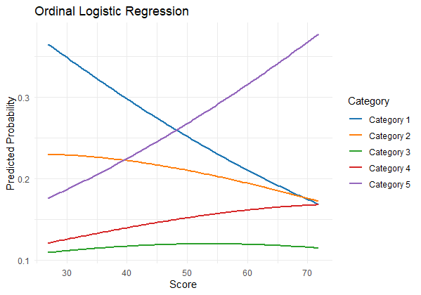
Ordinal Logistic Regression in R

• We use ggplot2 to create the visualization:
• We specify the predicted_probs dataframe as the data source.
• We create separate lines for each category’s predicted probability using geom_line.
• We set labels for the title, x-axis, and y-axis using labs.
• We customize the line colors using scale_color_manual and provide a legend title.
• We apply the “minimal” theme using theme_minimal() for a clean and simple appearance

Ordinal Logistic Regression on an Inbuilt Dataset

Pre-Requisites

Before moving forward make sure you have ordinal Package installed.

install.packages('ordinal')

• ordinal Package: Used for implementation of cumulative link (mixed) models also known as ordered regression models, proportional odds models, proportional hazards models

Loading Packages

R

library(ordinal)

Model Building

R

# Load the mtcars dataset
data(mtcars)

# Convert 'cyl' to an ordered factor
mtcars$cyl <- factor(mtcars$cyl, ordered = TRUE)

# Fit an ordinal logistic regression model
model <- clm(cyl ~ mpg + hp, data = mtcars)

• We load the ordinal package.
• We load the mtcars dataset and convert the cyl variable to an ordered factor as before.
• We fit an ordinal logistic regression model using the clm() function from ordinal package.
• Formula: cyl ~ mpg + hp – This indicates the formula used in the regression model. You are predicting the ordinal response variable cyl (number of cylinders) based on the predictor variables mpg (miles per gallon) and hp (horsepower).

Interpreting Model Results

R

summary(model)

Output:

formula: cyl ~ mpg + hp
data:    mtcars
 link  threshold nobs logLik AIC  niter max.grad cond.H 
 logit flexible  32   -0.00  8.00 30(1) 3.87e-09 1.1e+11
Coefficients:
    Estimate Std. Error z value Pr(>|z|)
mpg  -268.65         NA      NA       NA
hp     42.81         NA      NA       NA
Threshold coefficients:
    Estimate Std. Error z value
4|6    -1061         NA      NA
6|8     2232         NA      NA

• Link Function: logit – The link function used in ordinal logistic regression is the logit link function. It models the log-odds of an observation being in or below a particular category of the ordinal response variable.
• Threshold Function: flexible – The threshold function used is “flexible.” The threshold function defines how the categories of the ordinal response variable are separated based on the linear combination of predictor variables.
• Number of Observations (nobs): 32 – This indicates the number of observations in your dataset.
• Log Likelihood: -0.00 – The log-likelihood is a measure of how well the model fits the data. A higher log-likelihood indicates a better fit. In your case, the log-likelihood is very close to zero.
• AIC (Akaike Information Criterion): 8.00 – The AIC is a measure of the model’s goodness of fit, accounting for model complexity. Lower AIC values indicate a better balance between model fit and complexity.
• Number of Iterations (niter): 30(1) – This shows the number of iterations performed during the fitting process. It’s followed by (1), which typically indicates that the optimization algorithm successfully converged.
• Maximum Gradient (max.grad): 3.87e-09 – This is a measure of how much the log-likelihood function changed in the last iteration. A small value like this indicates that the optimization process has converged.
• Condition Number (cond.H): 1.1e+11 – The condition number is a measure of how well the predictor variables are scaled. A high condition number may indicate potential collinearity issues.
• Coefficients: The coefficient estimates for the predictor variables mpg and hp are shown in the “Estimate” column. However, there are missing values (NA) in the “Std. Error,” “z value,” and “Pr(>|z|)” columns. This may be due to issues such as perfect separation or multicollinearity in the data, which can lead to estimation problems in the model.
• Threshold Coefficients: These coefficients indicate the thresholds that separate different categories of the ordinal response variable. For example, the coefficient -1061 corresponds to the threshold between 4 and 6 cylinders, and 2232 corresponds to the threshold between 6 and 8 cylinders.

Conclusion

In conclusion, this article introduced ordinal logistic regression, a statistical technique for modelling outcomes that fall into an ordinal categorical category and have a natural order. We talked about the model’s fundamental ideas, when to use them, and the formula that was employed.

With an emphasis on coefficient estimates and threshold parameters, we gave concrete examples of fitting ordinal logistic regression models in R and deriving meaning from the findings. The reader will have a solid understanding of ordinal logistic regression after reading this article, enabling them to use it successfully to analyse data with ordered categories.