OpenCV Selective Search For Object Detection

OpenCV is a Python library that is used to study images and video streams. It basically extracts the pixels from the images and videos (stream of image) so as to study the objects and thus obtain what they contain. It contains low-level image processing and high-level algorithms for object detection, feature matching etc.

In this article, we will dive into a computer vision technique i.e. selective search for Object Detection in OpenCV.

Object Detection

Object Detection is a fundamental computer vision task that involves identifying and localizing objects or specific features within an image or a video stream. It plays a crucial role in numerous applications, including autonomous driving, surveillance, robotics, and image analysis. Object detection goes beyond mere object recognition by providing both the classification of objects into predefined categories or classes and the precise localization of where these objects exist within the image.

Sliding Window Algorithm

The sliding Window Algorithm is one of the important steps in Object detection algorithms. In the sliding window algorithm, we select a path or a region of the image by sliding a window or box over it and then classify each region that the window covers using an object recognition model. Over the course of the image, every object is thoroughly searched for. We must not only look at every available spot on the image but also at various scales. This is the case because many times object recognition models are trained on a certain set of scales. As a result, classification is required for many image regions or patches.

But the issue still persists. For objects with a fixed ratio, such as faces or people, the sliding window algorithm works well. According to the angle, the features of the objects can change dramatically. But when we search for different aspect ratios, this approach is a little more expensive.

Region Proposal Algorithm

The problem in the sliding window algorithm can be addressed using the region proposal algorithm. With the use of this technique, areas of a picture that are likely to contain objects are encapsulated by the bounding boxes. These region proposals typically contain proposals that nearly resemble the real object’s position, even though they occasionally may be noisy, overlapping or improperly aligned with those boundaries. The classification of these recommendations can then be done using object recognition models. The location of perspective objects is detected in areas with high probability.

In order to do this, the region proposal algorithm uses segmentation, which groups neighbouring image regions with comparable properties. The sliding window strategy, in contrast, looks for objects at all pixels places and sizes. Instead, these algorithms divide images into fewer regions, producing a much lower number of categorization suggested options. To allow for possible differences in object size and shape, these generated ideas are available in a range of scales and aspect ratios.

Region proposal method aims for high recall, prioritizing inclusion of regions with objects. This may result in number of proposals, including the false positives. While this can increase processing time and slight affect accuracy, its crucial to avoid missing actual objects, making high recall a valuable priority in object detection.

Selective Search

Selective Search is a region-based technique extensively used for object detection tasks within computer vision. It aims to generate a varied set of region proposals from an input image, where each region proposal representing a potential object or object portion.These region proposals are subsequently used as candidate regions by object detection algorithms to categorize and localize objects within an image.

Let’s understand that the how Selective Search algorithms works?

1. Image Segmentation: The process begins with the over-segmentation of the input image. Over-segmentation involves dividing the image into many smaller regions or superpixels. This initial segmentation is often performed using graph-based algorithms like the one by Felzenszwalb and Huttenlocher. The result is an initial set of small regions.
2. Region Grouping: Selective Search employs a hierarchical grouping approach. It begins with the initial small regions and progressively merges regions that are similar in terms of color, texture, size, and shape compatibility. The similarity between regions is determined using various image features.
3. Bounding Box Proposals: During the grouping process, bounding boxes of various sizes and aspect ratios are generated for each region. These bounding boxes represent the potential object candidates within those regions.
4. Training: The algorithm iteratively refines the grouping and generates more bounding box proposals by merging and splitting regions. This iterative approach continues until the satisfactory set of region proposals is obtained.
5. Output: The final output of Selective Search is a list of region proposals, each associated with a bounding box. These region proposals are used as candidate regions for subsequent object detection and recognition algorithms.

Similarity Measures

Similarity in Selective Search refers to the degree of visual resemblance between neighboring image regions based on color, texture, shape, and size. By quantifying these similarities using appropriate metrics, the algorithm groups regions that are likely to belong to the same object or object part, resulting in a hierarchical set of object proposals that can be used for further analysis and object detection tasks.

Now, lets look into different kinds of similarities:

Color Similarity: Color is one of the primary visual characteristics considered in Selective Search. Regions that have similar color distributions are more likely to belong to the same object. Mathematical illustration for color similarity to understand can be like in a color histogram of 25 bins is computed for each channel of the image and are concatenated to obtain a 25×3 = 75-dimensional color descriptor. It is based on histogram intersection between two regions and is calculated as below-

c_i^k is the histogram value for k^th bin in color descriptor.

Shape Similarity/Compatibility: The main idea behind shape compatibility is how better one image fits into the other one. The algorithm evaluates shape characteristics. Regions with similar shapes or contours might be grouped because objects often have consistent shapes. It is defined by the formula –

where size(BB_ij) is a bounding box around r_i and r_j .

Texture Similarity: Texture refers to the patterns or surface properties within an image region. Regions with similar textures, such as a smooth area or a region with a fine-grained texture, may be grouped together. To calculate the texture features, firstly gaussian derivatives are extracted at 8 orientations for each channel and then for each orientation and each color channel, a 10-bin histogram is computed resulting into a 10x8x3 = 240-dimensional feature descriptor. It is also calculated using histogram intersections –

t_i^k is the histogram value for k^th bin in texture descriptor.

Size Similarity: Regions of similar size might be more likely to belong to the same object or object part. It encourages smaller regions to merge early. By enforcing smaller regions to merge earlier, we can help prevent a large number of clusters from swallowing up all smaller regions. It is defined as –

where size(im) is size of image in pixels.

Final Similarity: The final similarity between two regions is defined as a linear combination of color similarity, texture similarity, size similarity, and shape similarity/compatibility.

Implementation of SelectiveSearch using python OpenCV

Let’s Manually build the Region for SelectiveSearch

Importing Libraries

Python3

# importing necessary libraries
import cv2
import selectivesearch
import matplotlib.pyplot as plt

Creation of bounding boxes Manually

Python3

# Load the image
image_path = 'img_1.jpg'
image = cv2.imread(image_path)
# Define bounding box coordinates (x, y, width, height)
bounding_boxes = [
    (100, 50, 200, 150),  # Example bounding box 1
    (300, 200, 150, 100),  # Example bounding box 2
    # Add more bounding boxes as needed
]

# Draw bounding boxes on the image
for (x, y, w, h) in bounding_boxes:
    cv2.rectangle(image, (x, y), (x + w, y + h), (0, 255, 0), 2)

# Display the image with bounding boxes
cv2_imshow(image)

# Wait for a key press and close the window
cv2.waitKey(0)
cv2.destroyAllWindows()

Output:

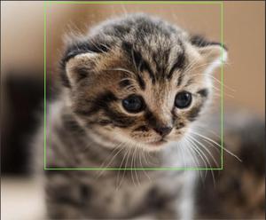
This bit of code shows how to load and display a picture with bounding boxes drawn around key areas. It specifies bounding boxes as tuples of (x, y, width, and height) coordinates and uses the OpenCV library (cv2) to read an image. The next step is to use cv2.rectangle() to create green rectangles around each location of interest on the image when the code loops over the list of bounding boxes. After using cv2_imshow() to display the image with bounding boxes, the software waits for a key press before destroying all open windows and releasing resources using cv2.waitKey(0) and cv2.destroyAllWindows().

Selective Search using Region proposals

We can use ‘selectivesearch.selective_search’ function to perform Selective Search on the image

Installing packages

pip install selectivesearch

Importing libraries

Python3

# importing necessary libraries
import cv2
import selectivesearch
import matplotlib.pyplot as plt

Loading image

Python3

# Load the image
image_path = 'elephant.jpg'
image = cv2.imread(image_path)

This code will load the image using openCV’s ‘imread’ function and stores it in the variable ‘image’.

Image Dimensions

Python3

# Print the dimensions of the loaded image
print(image.shape)
# Retrieve the width of the image
image.shape[1]
# Calculate the scaling factor for the image's height
(new_height / (image.shape[0]))

Here we are loading image and printing its dimensions, including height, width. Additionally it calculates the scaling factor for a new height based on a specified value.

Resize image to reduce computation time

Python3

# Calculate a new height
import matplotlib.pyplot as plt
new_height = int(image.shape[1] / 4)
# Calculate a new width
new_width = int(image.shape[0] / 2)
# Resize the image to the new dimensions
resized_image = cv2.resize(image, (new_width, new_height))

# Display the resized image using Matplotlib
plt.imshow(resized_image)
plt.show()

Output:

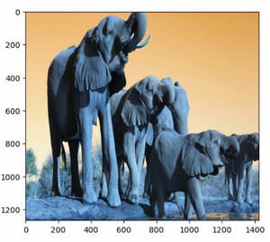
This code calculates new dimensions for an image based on specific proportions, resize the image accordingly, and then displays the resized image using matplotlib, resulting in a smaller representation of the original image.

Applying Search Selective on resized image

Python3

# applying selective search
img_lbl, regions = selectivesearch.selective_search(
    resized_image, scale=500, sigma=0.9, min_size=10)

“selectivesearch.selective_search” is a function provided by the selective search algorithm for object detection and image segmentation. This function performs a region proposal process on an input image to identify and generate potential regions of interests that may contain objects.
This code applies selective search algorithm to the resized image, aiming to generate region proposals for object detection. ‘Scale’ controls the trade off between the number of generated regions and their quality. Large values result in fewer regions but potentially higher quality. ‘Sigma’ value for gaussian function is used in smoothing the image. ‘min_size’ is the minimum size of a region proposal. Regions smaller than this are discarded.
After this, it performs the selective search and returns two main outputs i.e., ‘img_lbl’ contains the image labels and ‘regions’ contains the regions of interest generated by the algorithm. These regions represent potential objects in the image.

Calculating the Region

Python3

# Initialize an empty set to store selected region proposals
candidates = set()

# Iterate over all the regions detected by Selective Search
for r in regions:
    # Check if the current region's rectangle is already in candidates
    if r['rect'] in candidates:
        continue  # Skip this region if it's a duplicate

    # Check if the size of the region is less than 200 pixels
    if r['size'] < 200:
        continue  # Skip this region if it's too small

    # Extract the coordinates and dimensions of the region's rectangle
    x, y, w, h = r['rect']

    # Avoid division by zero by checking if height or width is zero
    if h == 0 or w == 0:
        continue  # Skip this region if it has zero height or width

    # Check the aspect ratio of the region (width / height and height / width)
    if w / h > 1.2 or h / w > 1.2:
        continue  # Skip this region if its aspect ratio is not within a range

    # If all conditions are met, add the region's rectangle to candidates
    candidates.add(r['rect'])

This code iterates through the regions generated by selective search, filtering and selecting regions based on specific criteria. It adds the valid regions to the candidates set. After the loop, it iterates over the detected regions.

Bounding Box Scaling

Python3

# Convert the selected bounding boxes to the original image size
candidates_scaled = [(int(x * (image.shape[1] / new_width)),
                      int(y * (image.shape[0] / new_height)),
                      int(w * (image.shape[1] / new_width)),
                      int(h * (image.shape[0] / new_height)))
                     for x, y, w, h in candidates]

return candidates_scaled

Here , in this code, it scales bounding boxes from a resized image back to their original dimensions, ensuring that regions of interest are accurately represented in the original image. It uses ratios between original and resized image dimensions for the scaling.

Search Selective for Object detection

Python3

# Load the image
image_path = 'elephant.jpg'
image = cv2.imread(image_path)

# Get selective search object proposals
proposals = selective_search(image)

# Draw the proposals on the image
output_image = image.copy()
for (x, y, w, h) in proposals:
    cv2.rectangle(output_image, (x, y), (x + w, y + h), (0, 255, 0), 20)

# Display the result
plt.imshow(output_image)
plt.show()

Output:

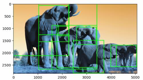
This code loads an image, applies selective search to generate object proposals, and then draws bounding boxes around these proposals on the image. Finally, it displays the image with the drawn bounding boxes.

Another Example

Python3

# Load the image from the specified path
image_path = 'dog.jpg'
image = cv2.imread(image_path)

# Get region proposals using Selective Search
proposals = selective_search(image)

# Create a copy of the original image to draw bounding boxes on
output_image = image.copy()

# Iterate through each region proposal and draw bounding boxes
for (x, y, w, h) in proposals:
    # Define the coordinates and dimensions of the bounding box
    x1, y1 = x, y  # Top-left corner
    x2, y2 = x + w, y + h  # Bottom-right corner

    # Draw a green bounding box around the region proposal on the output image
    cv2.rectangle(output_image, (x1, y1), (x2, y2), (0, 255, 0), 2)

# Display the result image with bounding boxes
plt.imshow(output_image)
plt.show()

Output:

Time complexity for this code is divided into different segments: Resizing of image, selective search, Iteration through different regions, scaling, drawing and showing up the results.

1. Resizing the image: O(H * W) where H and W are height and width respectively .
2. Selective Search Complexity: This time complexity is typically influenced by factors like the number of pixels, the scale parameter, and the complexity of region merging.
3. Iteration through regions: O(N) where N is number of regions.
4. Scaling: O(B), where B is the number of bounding boxes.
5. Drawing and showing up the result: O(B), where B is the number of bounding boxes.

Overall complexity would be the sum of all the complexities of sub categories i.e. O(H * W) + O(Selective Search) + O(N) + O(B) + O(B)

Application of Selective Search Algorithm in Object Detection

Selective search plays an important role in R-CNN(Region – based Convolutional Neural Network) family of the object detection models. It primary function is to efficiently generate a diverse set of region proposals, which are potential bounding boxes likely to contain objects within an image. This significantly reduces the computational burden by narrowing down the regions of interest for subsequent analysis. The generated region proposals are used as input to the R-CNN architecture, where they undergo feature extraction, classification and localization. High recall is a key benefit, ensuring that most potential object regions are included, even if some are false positives. R-CNN models then refine these proposals for accurate object localization. Ultimately, this collaboration between Selective Search and R-CNN model enhances both the efficiency and accuracy of object detection, making them suitable for real-time applications and complex scenes.