R-CNN | Region Based CNNs

Since Convolution Neural Network (CNN) with a fully connected layer is not able to deal with the frequency of occurrence and multi objects. So, one way could be that we use a sliding window brute force search to select a region and apply the CNN model to that, but the problem with this approach is that the same object can be represented in an image with different sizes and different aspect ratios. While considering these factors we have a lot of region proposals and if we apply deep learning (CNN) to all those regions that would computationally very expensive.

R-CNN architecture

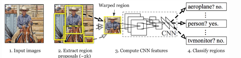
Ross Girshick et al in 2013 proposed an architecture called R-CNN (Region-based CNN) to deal with this challenge of object detection. This R-CNN architecture uses the selective search algorithm that generates approximately 2000 region proposals. These 2000 region proposals are then provided to CNN architecture that computes CNN features. These features are then passed in an SVM model to classify the object present in the region proposal. An extra step is to perform a bounding box regressor to localize the objects present in the image more precisely.

Region Proposals

Region proposals are simply the smaller regions of the image that possibly contains the objects we are searching for in the input image. To reduce the region proposals in the R-CNN uses a greedy algorithm called selective search.

Selective Search

Selective search is a greedy algorithm that combines smaller segmented regions to generate region proposals. This algorithm takes an image as input and output generates region proposals on it. This algorithm has the advantage over random proposal generation in that it limits the number of proposals to approximately 2000 and these region proposals have a high recall.

Algorithm

1. Generate initial sub-segmentation of the input image.
2. Combine similar bounding boxes into larger ones recursively
3. Use these larger boxes to generate region proposals for object detection.

In Step 2 similarities are considered based on color similarity, texture similarity, region size, etc. We have discussed the selective search algorithm in great detail in this article.

CNN architecture of R-CNN

After that these regions are warped into a single square of regions of dimension as required by the CNN model. The CNN model that we used here is a pre-trained AlexNet model, which is the state-of-the-art CNN model at that time for image classification Let’s look at AlexNet architecture here. 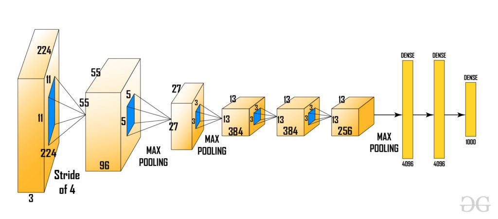Here the input of AlexNet is (227, 227, 3). So, if the region proposals are small and large then we need to resize that region proposal to given dimensions.

From the above architecture, we remove the last softmax layer to get the (1, 4096) feature vector. We pass this feature vector into SVM and bounding box regressor.

SVM (Support Vector Machine)

The feature vector generated by CNN is then consumed by the binary SVM which is trained on each class independently. This SVM model takes the feature vector generated in previous CNN architecture and outputs a confidence score of the presence of an object in that region. However, there is an issue with training with SVM is that we required AlexNet feature vectors for training the SVM class. So, we could not train AlexNet and SVM independently in paralleled manner. This challenge is resolved in future versions of R-CNN (Fast R-CNN, Faster R-CNN, etc.).

Bounding Box Regressor

In order to precisely locate the bounding box in the image., we used a scale-invariant linear regression model called bounding box regressor. For training this model we take as predicted and Ground truth pairs of four dimensions of localization. These dimensions are (x, y, w, h) where x and y are the pixel coordinates of the center of the bounding box respectively. w and h represent the width and height of bounding boxes. This method increases the Mean Average precision (mAP) of the result by 3-4%. 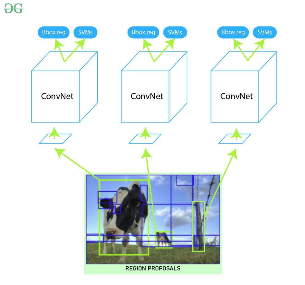Output:

Now we have region proposals that are classified for every class label. In order to deal with the extra bounding box generated by the above model in the image, we use an algorithm called Non- maximum suppression. It works in 3 steps:

• Discard those objects where the confidence score is less than a certain threshold value( say 0.5).
• Select the region which has the highest probability among candidates regions for the object as the predicted region.
• In the final step, we discard those regions which have IoU (intersection Over Union) with the predicted region over 0.5.

After that, we can obtain output by plotting these bounding boxes on the input image and labeling objects that are present in bounding boxes. 

Results

The R-CNN gives a Mean Average Precision (mAPs) of 53.7% on VOC 2010 dataset. On 200-class ILSVRC 2013 object detection dataset it gives an mAP of 31.4% which is a large improvement from the previous best of 24.3%. However, this architecture is very slow to train and takes ~ 49 sec to generate test results on a single image of the VOC 2007 dataset.

Challenges of R-CNN

• The selective Search algorithm is very rigid and there is no learning happening in that. This sometimes leads to bad region proposal generation for object detection.
• Since there are approximately 2000 candidate proposals. It takes a lot of time to train the network. Also, we need to train multiple steps separately (CNN architecture, SVM model, bounding box regressor). So, This makes it very slow to implement.
• R-CNN can not be used in real-time because it takes approximately 50 sec to test an image with a bounding box regressor.
• Since we need to save feature maps of all the region proposals. It also increases the amount of disk memory required during training.