LightGBM Feature parameters

LightGBM (Light gradient-boosting machine) is a gradient-boosting framework developed by Microsoft, known for its impressive performance and less memory usage. In this article, we’ll explore LightGBM’s feature parameters while working with the Wisconsin Breast Cancer dataset.

What is LightGBM?

Microsoft’s LightGBM (Light Gradient Boosting Machine) is an open-source, distributed, high-performance gradient boosting system. It is intended for the efficient training of large-scale machine learning models, and it works especially well with datasets with a huge number of features and samples.

What makes LightGBM special is its ability to work quickly and efficiently, even with large datasets. It uses techniques like:

• Gradient-based One Side Sampling (GOSS) to speed up training by focusing on the most important data points.
• Exclusive Feature Bundling (EFB) groups related features together, making it easier for the model to learn patterns.

Plus, LightGBM’s leaf split (best-first) strategy, by selecting a leaf with max delta loss to grow helps to create decision trees efficiently with lower loss compared to the level-wise algorithm.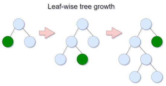

Feature Parameters in LightGBM

LightGBM provides a large set of parameters that can be tuned to control various aspects of model training and prediction.

Let’s explore some of the commonly used feature parameters and their use cases:

1. boosting (default gbdt)

It determines the boosting strategy used during model training.

• gbdt (Gradient Boosting Decision Tree): It utilizes traditional gradient boosting technique with decision trees as base learners.
• dart (Dropouts meet Multiple Additive Regression Trees): At each boosting iteration, it drops out (ignores) some trees randomly. This dropout helps prevent overfitting and mostly provides a better accuracy. We can further control dart using these parameters:
  • drop_rate (0 to 1.0): a fraction of trees to drop.
  • max_drop: max number of dropped trees during one boosting iteration.
  • skip_drop (0 to 1.0): probability of skipping the dropout procedure during a boosting iteration
  • drop_seed: random seed to choose dropping models
• rf: Random Forest builds trees independently and combines their predictions.

2. data_sample_strategy (default bagging)

The data_sample_strategy is like a tool to pick which data to learn from.

• bagging (Randomly Bagging Sampling): It’s like taking random samples of your data and learning from them. For manipulating the default bagging to you can change these parameters:
  • bagging_freq > 0
  • bagging_fraction < 1.0
• goss (Gradient-based One-Side Sampling): GOSS is a clever method that picks data points based on their importance. It focuses more on the samples with big gradients, which are the ones that can teach your model the most. Just like bagging you can modify the goss using these parameters:
  • top_rate: Retain ratio of large gradient data.
  • bottom_rate: Retain ratio of small gradient data.

3. learning_rate

It determines the step size at which the model updates its parameters during training.

A smaller learning rate, like 0.01, means tiny steps, so model learns slowly but might get very accurate. A larger learning rate, like 0.1, means bigger steps, so it learns faster but could miss the optimal solution.

4. objective (default regression)

There are many objectives, we are listing most commonly used:

• regression: The model predicts a continuous value, such as predicting the price of a house based on its features.

• binary: In binary classification, LightGBM uses Logistic regression, the model predicts one of two classes, something like “yes” or “no”, “Male” or “Female” etc.

5. num_iterations (default 100)

How many boosting iterations the model should go through during training.

6. metric (default = “”)

To specify the evaluation metric used during the model training process to assess its performance. You can provide a single metric or a list of metrics for evaluation like ‘metrics’: [‘auc’, ‘binary_logloss’]

When metric is set to an empty string (“”), or not specified, LightGBM automatically uses the metric corresponding to the specified objective. For example, if your objective is “binary,” it will use “binary_logloss” as the evaluation metric.

Some commonly used evaluation metrics in LightGBM:

For classification tasks:

• auc: Area Under the Receiver Operating Characteristic Curve (AUC).
• binary_logloss: Logarithmic loss for binary classification.
• map: Mean Average Precision.

For regression tasks:

• l1: Absolute loss or mean absolute error.
• l2: Square loss or mean squared error.
• rmse: Root mean squared error.

7. max_depth

This parameter limits the maximum depth of the decision trees. Setting it to a positive integer restricts the depth, which can prevent the trees from becoming overly complex and overfitting the data. If you want the trees to grow without restrictions, set it to -1.

8. num_leaves (default 31)

Maximum number of leaves in single decision tree. Increasing num_leaves creates more complex trees, but they can overfit on smaller datasets. Reducing num_leaves simplifies trees, making them less prone to overfitting but losing some details.

9. min_data_in_leaf

This parameter specifies the minimum number of data points required in a leaf node. It helps to deal with overfitting by ensuring that each leaf contains a minimum amount of data. Smaller values make the model more prone to overfitting, while larger values prevent excessive partitioning.

10. max_bin

The max_bin parameter in LightGBM controls the maximum number of bins in which feature values are divided or “bucketed.”

Smaller values for max_bin result in fewer bins and may lead to less precise training, but they can enhance the model’s generalization capabilities, making it more resistant to overfitting. Larger values, on the other hand, provide more detailed representations of the data but can increase the risk of overfitting.

11. bagging_fraction

Bagging, or random sampling of the data, can help prevent overfitting. You can use this parameter to control what fraction of the data is used for each training iteration. Reducing it to less than 1.0 means that only a portion of the data is used, introducing randomness and reducing the risk of overfitting.

12. feature_fraction

Similar to bagging, you can randomly select a subset of features for each tree during training. If you set feature_fraction to a value less than 1.0, it helps reduce overfitting by limiting the features used for each tree, introducing diversity.

13. extra_trees

Enabling “extra_trees” builds extremely randomized trees. In these trees, during node splits, LightGBM will check only one randomly-chosen threshold for each feature. This randomness can help prevent overfitting by making the trees less sensitive to individual data points.

Implementing LightGBM

We will implement LightGBM, using the lightgbm Python package. To get started, make sure you have LightGBM installed by running the following command in your terminal:

pip install lightgbm

Next we are importing the necessary sklearn functions for loading and splitting the dataset and measuring classification accuracy.

Importing Libraries

Let’s start by importing the necessary libraries, loading the Wisconsin Breast Cancer dataset and splitting it into train and test data:

Python3

import lightgbm as lgb
from sklearn.datasets import load_breast_cancer
from sklearn.model_selection import train_test_split
from sklearn.metrics import accuracy_score

Loading Breast Cancer dataset and splitting it into train and test data

Python

# Load the dataset
data = load_breast_cancer()
X, y = data.data, data.target

# Split the data into training and testing sets
X_train, X_test, y_train, y_test = train_test_split(X, y, test_size=0.2, random_state=42)

We load the dataset with the load_breast_cancer() function. This dataset is commonly utilized for binary classification tasks, where the objective is to distinguish between malignant and benign tumors. After this, using train_test_split we are splitting the dataset into 80% train data and 20% test data.

Defining hyperparameters for LightGBM

Python

# Define LightGBM parameters
params = {
    'boosting': 'gbdt',
    'objective': 'binary',
    'metric': 'binary_logloss',  # You can use other metrics as well
    'num_leaves': 45,
    'learning_rate': 0.1,
    'max_depth': 5,
    'min_data_in_leaf': 20,
    'max_bin': 255,
    'bagging_fraction': 0.8,
    'feature_fraction': 0.8
}

Here we are defining the parameters to use with our LightGBM model:

• The boosting parameter is set to ‘gbdt’, indicating the use of default gradient boosting.
• The objective is specified as ‘binary’ since we are dealing with a binary classification task.
• The metric is set to ‘binary_logloss,’ which calculates the logarithmic loss for binary classification.
• Hyperparameters such as num_leaves control the complexity of individual trees, and learning_rate determines the step size during model updates.
• Parameters like max_depth, min_data_in_leaf, and max_bin are set to manage overfitting and tree depth.
• The parameters bagging_fraction and feature_fraction introduce randomness by using only a fraction of the data and features during training, aiding in preventing overfitting..

Creating a LightGBM dataset

Python

train_data = lgb.Dataset(X_train, label=y_train)

This step is necessary for preparing the data in a format suitable for LightGBM’s training process. We are providing the training data as X_train and the training labels as y_train to generate train_data suitable for training LightGBM model.

Step 5: Train the model

Python

num_boost_round = 100  # You can adjust the number of boosting rounds
model = lgb.train(params, train_data, num_boost_round=num_boost_round)

The model is trained using the train method in which we pass, parameters specified earlier (params) and the LightGBM dataset (train_data) we created.

The num_boost_round parameter allows us to control the number of boosting rounds or iterations, influencing the model’s learning process. Try changing the num_boost_round parameter to gain insights into its impact on overfitting.

Step 6: Make predictions on the test set

Python

# Make predictions on the test set
y_pred = model.predict(X_test)
y_pred_binary = [1 if pred > 0.5 else 0 for pred in y_pred]

We use the trained model to predict the likelihood of each sample in the test set belonging to the positive class (in our case, indicating a malignant tumor).

The model outputs a probability score for each sample. To convert these scores into actual predictions, we set a threshold of 0.5.

If the predicted probability is higher than 0.5, we label the sample as 1 (positive), indicating a prediction for a malignant tumor. If it’s below 0.5, we label it as 0 (negative), suggesting a benign tumor.

Step 7: Evaluate the model

Accuracy score

Python

accuracy = accuracy_score(y_test, y_pred_binary)
print(f"Accuracy: {accuracy}")

Output:

Accuracy: 0.9736842105263158

We have achieved an accuracy of approximately 97.37% signifying that the model correctly predicted the nature of breast tumors for the majority of the test set.

Classification report

Python

from sklearn.metrics import classification_report, confusion_matrix

# Classification Report
print("Classification Report:")
print(classification_report(y_test, y_pred_binary))

Output:

Classification Report:
              precision    recall  f1-score   support

           0       0.98      0.95      0.96        43
           1       0.97      0.99      0.98        71

    accuracy                           0.97       114
   macro avg       0.97      0.97      0.97       114
weighted avg       0.97      0.97      0.97       114

For class 0 (benign tumors), the F1 score of 96% reflects a balanced performance in terms of precision and recall, pointing to the model’s ability to accurately identify and minimize false positives for benign cases. Similarly, for class 1 (malignant tumors), the F1 score of 98% demonstrates the model’s capability in correctly identifying malignant cases.

Confusion matrix

Python

import seaborn as sns
import matplotlib.pyplot as plt

# Confusion Matrix
cm = confusion_matrix(y_test, y_pred_binary)

# Plot Confusion Matrix using Seaborn
sns.heatmap(cm, annot=True, fmt="d", cbar=False,
            xticklabels=["Benign (0)", "Malignant (1)"],
            yticklabels=["Benign (0)", "Malignant (1)"])
plt.xlabel("Predicted")
plt.ylabel("True")
plt.title("Confusion Matrix")
plt.show()

Output:

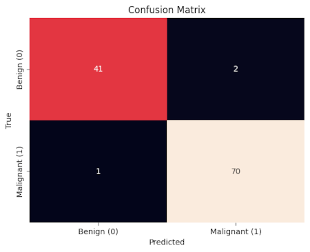
The model correctly identified 41 benign tumors and 70 malignant tumors, with only 1 benign tumor misclassified as malignant and 2 malignant tumors misclassified as benign.

Conclusion

LightGBM is a powerful tool that lets us build machine learning models. It’s also great for beginners because it’s user-friendly. Feature parameters help us control how our model learns, try doing hyperparameter tuning to find the perfect model for your task.