How to approach a Machine Learning project : A step-wise guidance

This article will provide a basic procedure on how should a beginner approach a Machine Learning project and describe the fundamental steps involved. In the problem, we will focus on the classification of iris flowers. You can learn about the dataset here.

Many teachers and websites take up this problem to demonstrate the various nuances involved in a Machine Learning project because –

1. All the attributes are numeric and all the attributes are of same scale and units.
2. The problem in hand is a classification problem and thus gives us an option to explore many evaluation metrics.
3. The dataset involved is a small and clean and thus can be handled easily.

We demonstrate the following steps and describe them accordingly along the way. 

Step 1: Importing the required libraries

Python3

import pandas as pd
from pandas.plotting import scatter_matrix
import matplotlib.pyplot as plt
from sklearn import model_selection
from sklearn.metrics import classification_report, confusion_matrix, accuracy_score
from sklearn.linear_model import LogisticRegression
from sklearn.tree import DecisionTreeClassifier
from sklearn.neighbors import KNeighborsClassifier

Step 2: Loading the Data

Python3

# dataset (csv file) path
url = "https://raw.githubusercontent.com /jbrownlee/Datasets/master/iris.csv"

# selectng necessary feature
features = ['sepal-length', 'sepal-width', 'petal-length', 'petal-width', 'class']

# reading the csv
data = pd.read_csv(url, names = features)

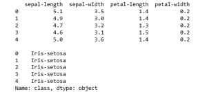
Step 3: Summarizing the Data

This step typically involves the following steps-

a) Taking a peek at the Data

Python3

data.head()

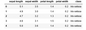
b) Finding the dimensions of the Data

Python3

data.shape

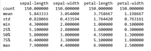
c) Statistical summary all attributes

Python3

print(data.describe())

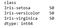
d) Class distribution of the Data

Python3

print((data.groupby('class')).size())

Step 4: Visualising the Data 
This step typically involves the following steps –

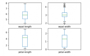
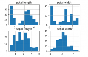
a) Plotting Univariate plots
This is done to understand the nature of each attribute.

Python3

data.plot(kind ='box', subplots = True, layout =(2, 2),
                       sharex = False, sharey = False)

plt.show()

Python3

data.hist()
plt.show()

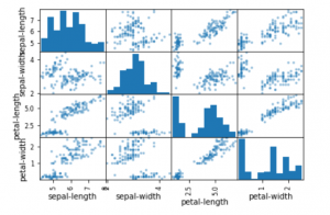
b) Plotting Multivariate plots
This is done to understand the relationships between different features.

Python3

scatter_matrix(data)
plt.show()

Step 5: Training and Evaluating our models
This step typically contains the following steps –

a) Splitting the training and testing data
This is done so that some part of the data is hidden from the learning algorithm

Python3

y = data['class']
X = data.drop('class', axis = 1)
X_train, X_test, y_train, y_test = model_selection.train_test_split(
                           X, y, test_size = 0.25, random_state = 0)

print(X.head())
print('')
print(y.head())

b) Building and Cross-Validating the model

Python3

algorithms = []
scores = []
names = []

algorithms.append(('Logistic Regression', LogisticRegression()))
algorithms.append(('K-Nearest Neighbours', KNeighborsClassifier()))
algorithms.append(('Decision Tree Classifier', DecisionTreeClassifier()))

for name, algo in algorithms:
    k_fold = model_selection.KFold(n_splits = 10, random_state = 0)

    # Applying k-cross validation
    cvResults = model_selection.cross_val_score(algo, X_train, y_train,
                                      cv = k_fold, scoring ='accuracy')

    scores.append(cvResults)
    names.append(name)
    print(str(name)+' : '+str(cvResults.mean()))

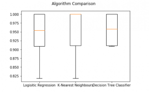
c) Visually comparing the results of the different algorithms

Python3

fig = plt.figure()
fig.suptitle('Algorithm Comparison')
ax = fig.add_subplot(111)
plt.boxplot(scores)
ax.set_xticklabels(names)
plt.show()

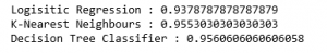
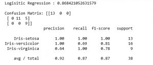
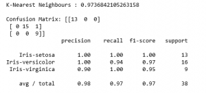
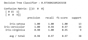
Step 6: Making predictions and evaluating the predictions

Python3

for name, algo in algorithms:
    clf = algo
    clf.fit(X_train, y_train)
    y_pred = clf.predict(X_test)
    pred_score = accuracy_score(y_test, y_pred)

    print(str(name)+' : '+str(pred_score))
    print('')
    print('Confusion Matrix: '+str(confusion_matrix(y_test, y_pred)))
    print(classification_report(y_test, y_pred))

Reference – https://machinelearningmastery.com/machine-learning-in-python-step-by-step/