Hebbian Learning Rule with Implementation of AND Gate

Hebbian Learning Rule, also known as Hebb Learning Rule, was proposed by Donald O Hebb. It is one of the first and also easiest learning rules in the neural network. It is used for pattern classification. It is a single layer neural network, i.e. it has one input layer and one output layer. The input layer can have many units, say n. The output layer only has one unit. Hebbian rule works by updating the weights between neurons in the neural network for each training sample.

Hebbian Learning Rule Algorithm : 

1. Set all weights to zero, w_i = 0 for i=1 to n, and bias to zero.
2. For each input vector, S(input vector) : t(target output pair), repeat steps 3-5.
3. Set activations for input units with the input vector X_i = S_i for i = 1 to n.
4. Set the corresponding output value to the output neuron, i.e. y = t.
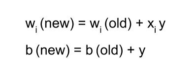
5. Update weight and bias by applying Hebb rule for all i = 1 to n:

Implementing AND Gate : 

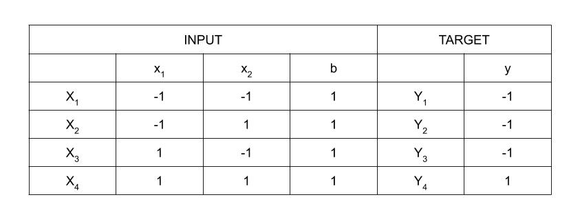
Truth Table of AND Gate using bipolar sigmoidal function

There are 4 training samples, so there will be 4 iterations. Also, the activation function used here is Bipolar Sigmoidal Function so the range is [-1,1]. 

Step 1 : 

Set weight and bias to zero, w = [ 0 0 0 ]^T  and b = 0.

Step 2 : 

Set input vector X_i = S_i  for i = 1 to 4.

X₁ = [ -1 -1 1 ]^T

X₂ = [ -1 1 1 ]^T

X₃ = [ 1 -1 1 ]^T

X₄ = [ 1 1 1 ]^T

Step 3 : 

Output value is set to y = t.

Step 4 : 

Modifying weights using Hebbian Rule:

First iteration – 

w(new) = w(old) + x₁y₁ = [ 0 0 0 ]^T + [ -1 -1 1 ]^T . [ -1 ] = [ 1 1 -1 ]^T

For the second iteration, the final weight of the first one will be used and so on.

Second iteration –

w(new) = [ 1 1 -1 ]^T + [ -1 1 1 ]^T . [ -1 ] = [ 2 0 -2 ]^T

Third iteration – 

w(new) = [ 2 0 -2]^T + [ 1 -1 1 ]^T . [ -1 ] = [ 1 1 -3 ]^T

Fourth iteration – 

w(new) = [ 1 1 -3]^T + [ 1 1 1 ]^T . [ 1 ] = [ 2 2 -2 ]^T

So, the final weight matrix is [ 2 2 -2 ]^T

Testing the network : 

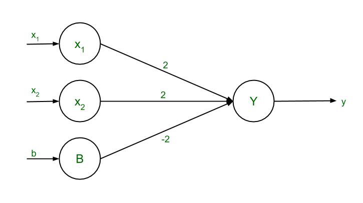
The network with the final weights

For x₁ = -1, x₂ = -1, b = 1, Y = (-1)(2) + (-1)(2) + (1)(-2) = -6

For x₁ = -1, x₂ = 1, b = 1, Y = (-1)(2) + (1)(2) + (1)(-2) = -2

For x₁ = 1, x₂ = -1, b = 1, Y = (1)(2) + (-1)(2) + (1)(-2) = -2

For x₁ = 1, x₂ = 1, b = 1, Y = (1)(2) + (1)(2) + (1)(-2) = 2

The results are all compatible with the original table.

Decision Boundary : 

2x₁ + 2x₂ – 2b = y

Replacing y with 0, 2x₁ + 2x₂ – 2b = 0

Since bias, b = 1, so 2x₁ + 2x₂ – 2(1) = 0

2( x₁ + x₂ ) = 2

The final equation, x₂ = -x₁ + 1

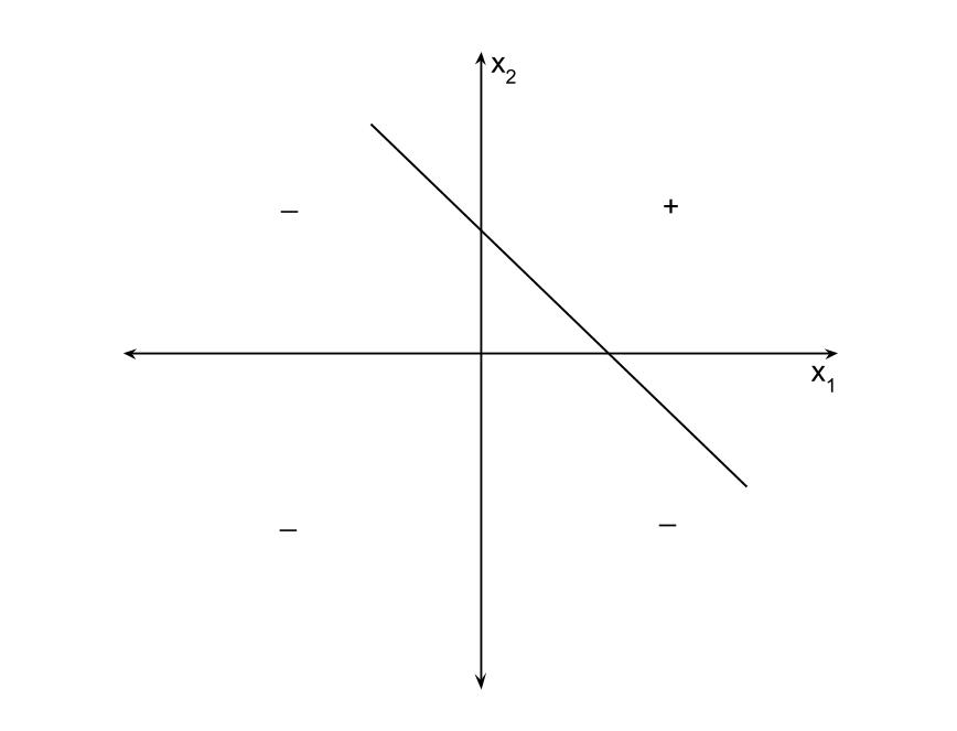
Decision Boundary of AND Function