Excel Formatting Shortcuts
If you have closely followed the previous parts of this tutorial, you already know most of the Excel formatting shortcuts. The table below provides a summary.
Shortcut Format
Ctrl+Shift+~ General format
Ctrl+Shift+! Number format with a thousand separators and two decimal places.
Ctrl+Shift+$ Currency format with two decimal places and negative numbers displayed in parentheses
Ctrl+Shift+% Percentage format with no decimal places
Ctrl+Shift+^ Scientific notation format with two decimal places
Ctrl+Shift+# Date format (dd-mmm-yy)
Ctrl+Shift+@ Time format (hh: mm AM/PM)
Excel opens with all the cells looking the same. Things can get hard to understand if you have a lot of them. Changing Excel’s look is as simple as changing the font and size parameters to modify the appearance of your written work. The key points become more apparent, and the material becomes more accessible.
Excel also lets you choose whether the numbers are money ($) or percentages (%). Then, it will know just what to display to them. After these easy changes, your Excel file will look better and be easier for everyone to understand.
How to Change the Font?
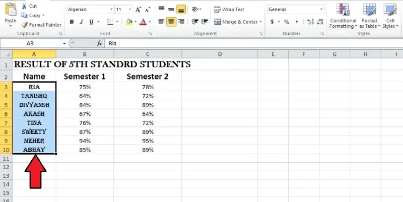
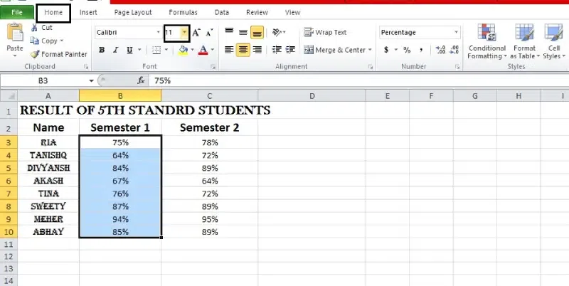
Step 1: Select the cell
Click on the cell or drag to select multiple cells where you want to change the font.
Select the cell
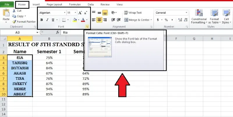
Step 2: Click the Font dropdown arrow
To access the Font menu, go to the Home tab and click the arrow near the dropdown.
Click the Font dropdown arrow
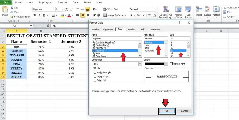
Step 3: Select the desired font
You can pick one from the list of available fonts.
Select the desired font
Step 4: The font will change
The text in the chosen cells will immediately change to reflect the new font style after you’ve picked a font.
How to Change the Font Size?
Step 1: Select the cells
Select the cell to change the font size of it.
Select the cells
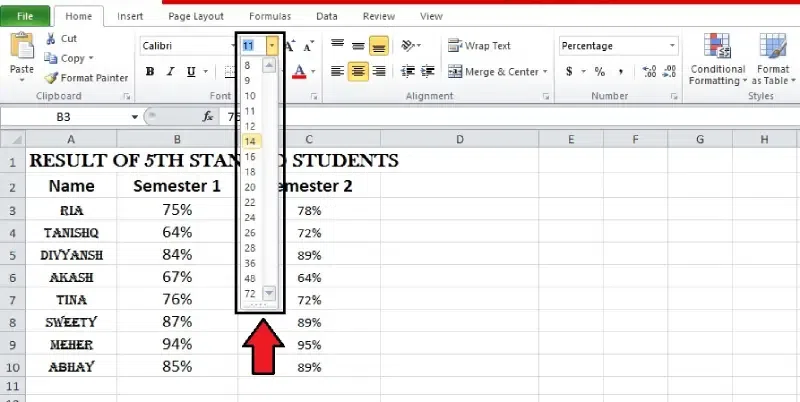
Step 2: Open Font Size dropdown
Click the dropdown arrow next to the Font Size command on the Home tab.
Open Font Size dropdown
Step 3: Select the font size
Select a font size from the list of available options.
Select the font size
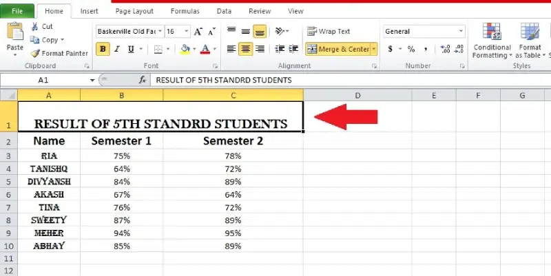
Step 4: Once applied, the text in the selected cells will be resized to match the font size.
Note: You may adjust the font size using the keyboard keys “Increase” and “Decrease” or by navigating the controls on your keyboard.
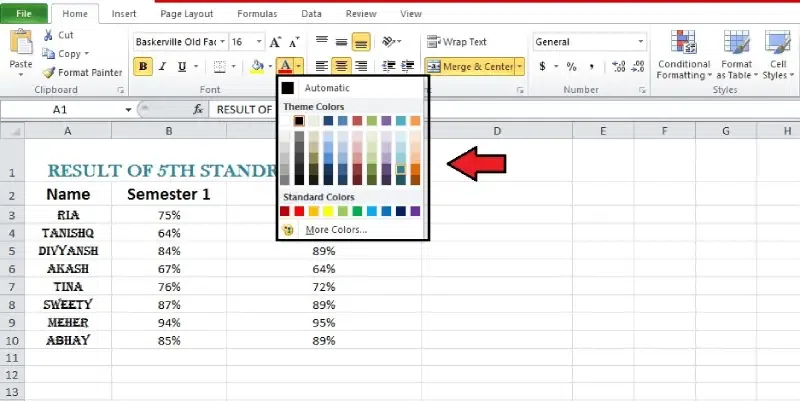
How to Change the Font Color?
Step 1: Select the cells
Click on one cell or drag to select multiple cells.
Select the cells
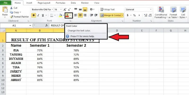
Step 2: Open the Font Color dropdown on Home
Simply click the down arrow next to Font Colour on the Home to change the font colour.
Open the Font Color dropdown on Home
Step 3: Select the font color
Pick a colour from the spectrum that works for you.
Select the font color
Step 4: The selected font colour will changed
The text in the chosen cells will be changed to match the new colour of the font.
How to Use the Bold, Italic, and Underline Commands?
Step 1: Select the cells
Press and hold or drag to choose several cells for formatting.
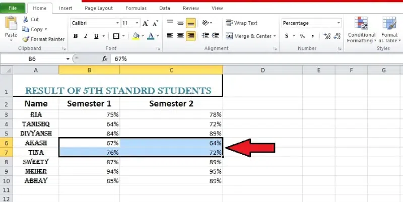
Select the cells
Step 2: Select Bold, Italic, or Underline from the Home
From the Home menu, choose Bold (B), Italic (I), or Underline (U). This will change the style of the text you have chosen.
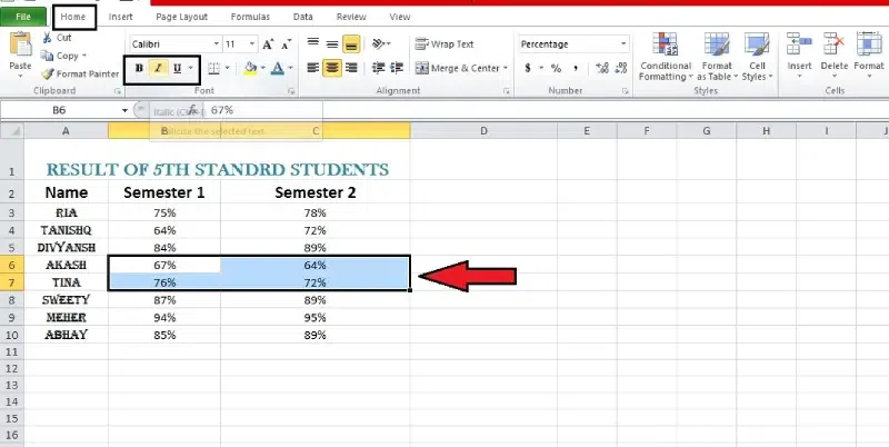
Select Bold, Italic, or Underline from the Home
Step 3: The selected style will be applied
The highlighted, italicised, or bolded text will be the one you choose.
Note: Pressing Ctrl+B, Ctrl+I, and Ctrl+U on the keyboard will correspondingly bold, italicise, and underline the chosen text.
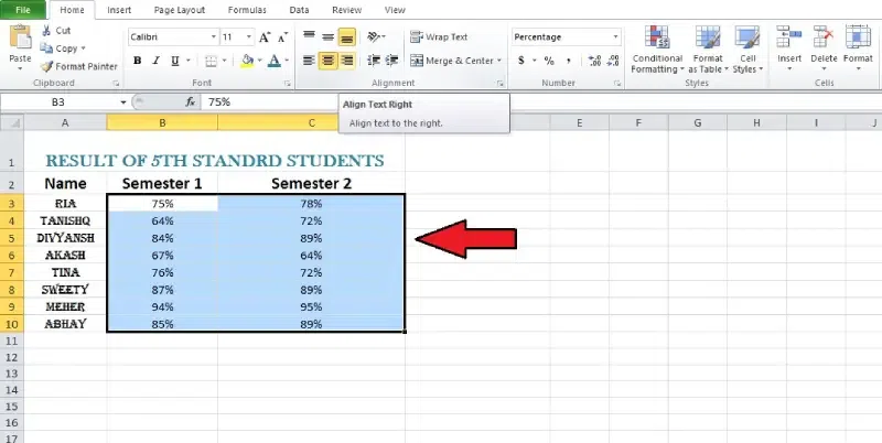
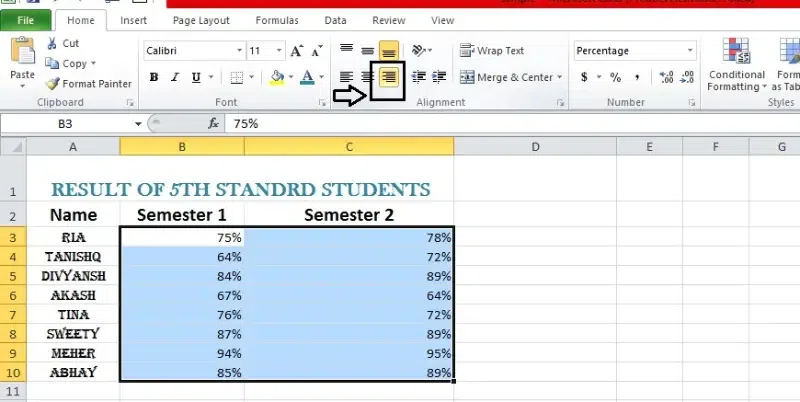
How to use Text Alignment?
Numbers will be aligned to the bottom-right of a cell and text to the bottom-left of a cell in your worksheet by default. You may arrange cell information to make it simpler to read.
Step 1: Select the cells
Click or drag to select multiple cells to change text alignment.
Select the cells
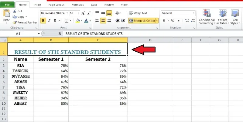
Step 2: Go to the Home, find alignment options
To access the Home tab in Excel, go to the ribbon. Various alignment choices may be found in the “Alignment” category.
Step 3: Choose from left, centre, or right alignment options
Choose one of the three horizontal alignment commands from the Home tab: left, centre, or right.
Go to the Home, find alignment options
Step 4: The text will realign
Text in the selected cells will be aligned after you make your selection.
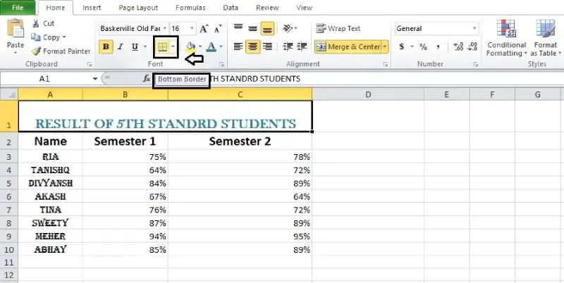
How To Add a Border in Excel?
Step 1: Select the cells
To add a border, click on the cell or groups of cells that you want to border.
Select the cells
Step 2: Click the Borders on the Home
On the Excel menu, go to the Home tab. The “Borders” button is in the “Font” group. It looks like a grid with borders.
Click the Borders on the Home
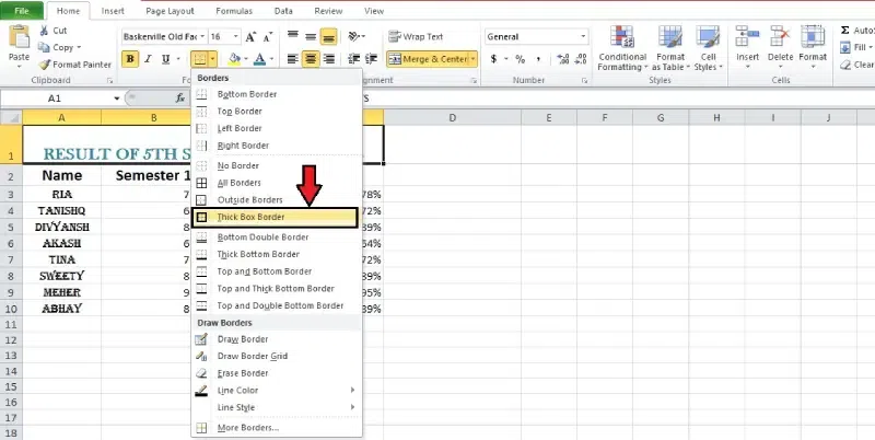
Step 3: Select the border style
From the dropdown box, pick the border style you want to use. Some options are: There are no borders, all borders, outside borders, thick box borders, and more borders.
Select the border style
Step 4: Apply Border
Click on the border style option to apply it to the selected cells.
How To Add a Fill Color?
Step 1: Select the cells
Click on the cell where you want to fill in the colour.
Select the cells
Step 2: Click “paint bucket” in the “Font” group
On the Excel menu, go to the Home tab. The “Fill Colour” button is in the “Font” group. Like a paint bucket, it usually has a colour label.
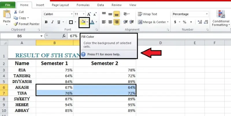
Click “paint bucket” in the “Font” group.
Step 3: Select the color
Please choose the colour you want to use as the fill colour by clicking on it in the palette.
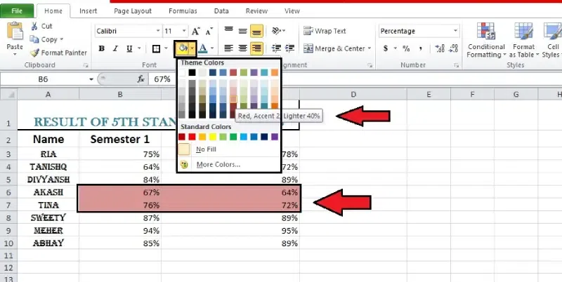
Select the color
Step 4: Click on it to apply
Choose a colour, and then the cells will be filled with that colour.
Applying formatting to several cells at once is easy with the Format Painter. Copying the formatting of a specific cell or range to another location in your spreadsheet is simple with this helpful function.
Step 1: Click on a cell with the style
Pick out the cell that features the style you wish to copy.
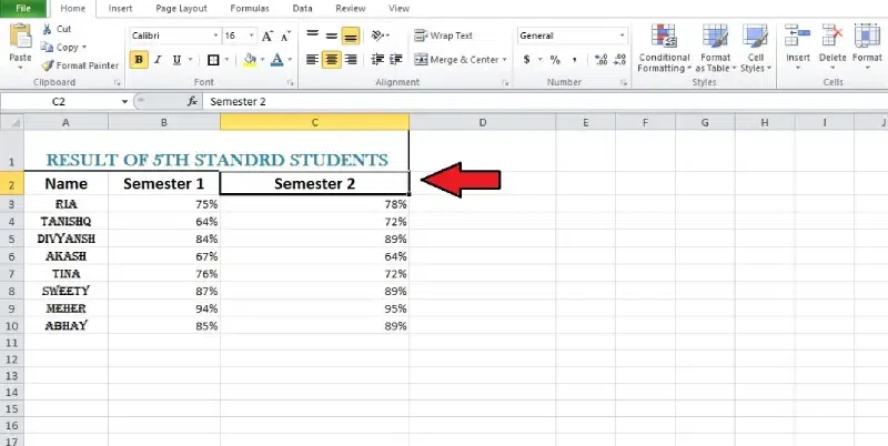
Click on a cell with the style
Step 2: Locate the Format Painter section at Home
Go to home and find the Format Painter section.
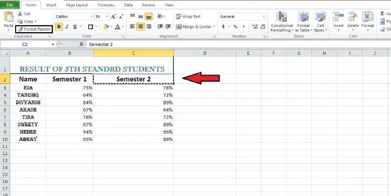
Locate the Format Painter section at Home
Step 3: Click on it
Click on the format painter when you find it.
Click on the format painter when you find it
Step 4: Click on the cell for the same style
Select the cells you want to format or a range of cells, and then click and drag to apply the style.
Step 1: Copy formatting from the first cell.
Like the other cell, the format of the selected one will be modified.
Cell Styles
Excel has built-in cell styles, so you can forget to manually format cells. Cell styles in Excel make it easy to professionally arrange the contents of cells, like titles and heads.
Step 1: Select the cells
Select cells where you want to apply a cell style.
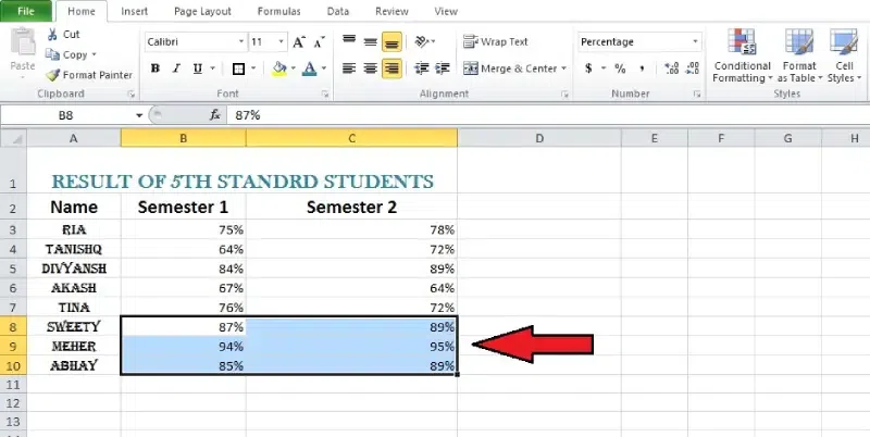
Select the cells
Step 2: Click the Styles on the Home
On Home, click Styles and choose the style from the dropdown menu.
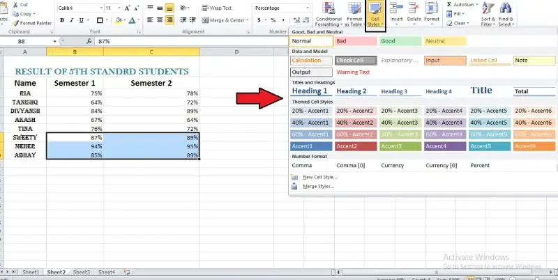
Click the Styles on the Home
Step 3: Select the style and press enter
Select a cell style and press enter to apply it to selected cells.
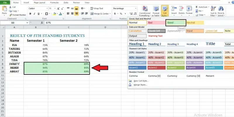
Select the style and press enter
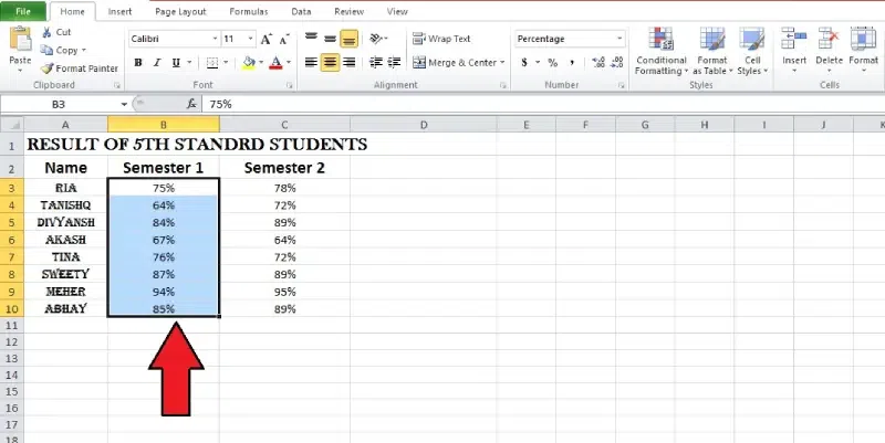
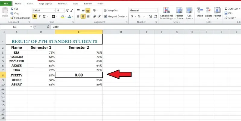
One of Excel’s powerful features is applying specific formatting to numbers. Formatting allows you to vary the look of dates, times, decimals, percentages, currency ($), and much more rather than presenting all cell information similarly.
Step 1: Select the cells
Select cells to apply formatting.
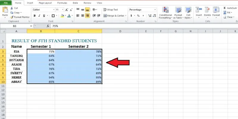
Select the cells
Step 2: Click the dropdown menu in the “Number” group
Click the dropdown menu in the “Number” group to choose a number format.
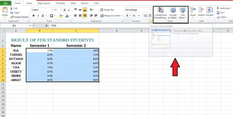
Click the dropdown menu in the “Number” group
Step 3: Select the Number format
Choose from the available choices (Date, Time, Currency, Percentage, etc.) by scrolling down the page.
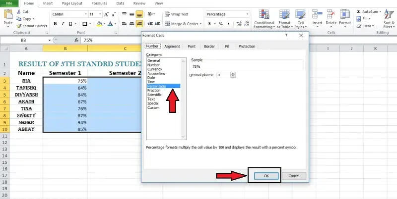
Select the Number format
Step 4: The selected formatting will be applied
Once you’ve chosen a formatting option, it will be applied to the selected cells.
Conclusion
Excel-style rules can help your data look better and be easier to understand. For neat and professional-looking spreadsheets, learn how to use the Format Painter, change fonts, sizes, and colours, align text, add borders and colours, and apply cell styles. The skills listed here make your work look better and help you organise knowledge so it’s easier to understand.
How do I auto-format cells in Excel?
You can use a method to make this whole process automatic. You can change the style by pressing Alt 0 A and clicking inside the table. Following that, Excel will automatically clean and arrange your data.
How do I format a lot of cells in Excel?
Pick the cell with your desired format, then press Ctrl+C to copy its contents and forms. Click on the column name or row you want to change the style to select the whole thing. To paste special, right-click on the pick and choose “Paste Special.” Click Formats in the Paste Special box, then click OK.
How do I conditionally format cells in Excel?
Click the down arrow under Conditional Formatting on the Home tab’s Style group, then choose Highlight Cells Rules. To use a specific command, such as “Between,” “Equal To,” or “A Date Occurring,” choose it. Type in the desired values and then choose a format.
Share your thoughts in the comments
Please Login to comment...