Linear Interpolation in Excel
Last Updated :
07 Mar, 2024
Linear interpolation is used for fitting curves using linear polynomials. Linear Interpolation is a method that constructs new data points from a given set of data points. Linear interpolation is useful when looking for a value between two data points. It can be considered as “filling in the gaps” in a table of data. The strategy for linear interpolation is to use a straight line to connect the known data points on either side of the unknown point. It finds the unknown values in the table. The formula of linear interpolation is given by,
Linear Interpolation Formula
[Tex]y = y_1 + (x-x_1)\frac{y_2-y_1}{x_2-x_1}[/Tex]
Where,
- x1 and y1 are the first coordinates, and
- x2 and y2 are the second coordinates
- x is the point to perform the interpolation
- y is the interpolated value
Linear Interpolation in Excel
We’ll be looking at two ways to calculate the Linear Interpolation in Excel.
Case 1: When we have 2 pairs of values for the x and y coordinates. For Example:
We want to check the value of 2.3 and hence we have to use interpolation. We are using linear interpolation because the values of x and y are changing linearly. We’ll be using the FORECAST formula,
=FORECAST(x, known_y’s, known_x’s)
Note: In Excel 2016, the FORECAST function was replaced with FORECAST.LINEAR. The syntax and usage of the two functions are the same.
Step 1: Add the FORECAST.LINEAR formula to the cell where you want to add the interpolated value.
Step 2: Fill the formula with the desired values. First, the value of x will go, then add the y-axis values and finally add x-axis values in the formula and click Enter. You’ll get the desired result.
Here the interpolated value of 2.3 is 5.6
Case 2: When we have more than 2 pairs of values for the x and y coordinates.
For Example, We have the data of rainfall (in cm) received in some parts of India for consecutive 7 days. We want to predict rainfall at 1.5 days.
First, we need to check x1, x2, y1, and y2. To perform this we will be using VLOOKUP, INDEX, and MATCH
VLOOKUP: It is used when you need to find things in a table or a range by row.
Syntax:
=VLOOKUP (lookup_value, table_array, col_index_num, [range_lookup])
range_lookup: It is an optional parameter. We can enter 1/True, which looks for an approximate match while 0/False, which looks for an exact match.
INDEX: It is used when you need a value or reference to a value from within a table or range.
Syntax:
= INDEX(array, row_num, [column_num])
Where array and row_num are required values and column_num is optional.
MATCH: This function searches for a specified item in a range of cells, and then returns the relative position of that item in the range.
Syntax:
= MATCH(lookup_value, lookup_array, [match_type])
Where lookup_value and lookup_array are required values and match_type is optional.
We will be calculating all the other values using the formulas above.
Step 1: Calculating x1 using VLOOKUP. Enter the formula and values as shown below.
Step 2: Press Enter and you’ll get the desired value (as shown below).
Step 3: Calculating y1 using VLOOKUP. Enter the formula and values as shown below. The only change we need to do here is the change in col_index_num to 2 because we want the values from column C.
Step 4: Press Enter and you’ll get the desired value (as shown below).
To calculate the values of x2 and y2, we’ll be using INDEX and MATCH functions.
Step 5: Calculate x2 using INDEX and MATCH functions. Enter the formula and values as shown below.
Step 6: Press Enter and you’ll get the desired value (as shown below).
Step 7: Calculate y2 using INDEX and MATCH functions. Enter the formula =INDEX($C$2:$C$8, MATCH(F6,$C$2:$C$8)+1) and values as shown below. The only change here is of Column C and the value of y1.
Step 8: Press Enter and you’ll get the desired value (as shown below).
Now, we’ll be using the above-mentioned formula to calculate the y value.
Step 9: Put all the calculated values in the formula in the desired cell. (as shown below)
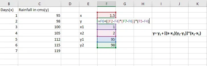
Step 10: Press Enter and you’ll get the desired results.

Share your thoughts in the comments
Please Login to comment...