How to Apply Conditional Formatting in a Pivot Table in Excel

One of the most useful ways to customize the pivot table formatting is using Conditional Formats. Conditional formatting rules can be applied to Pivot tables just like they can be applied to normal data ranges. So by using conditional formatting, we can highlight the cells with a certain color depending on the cell’s value.

Conditional Formatting

What is Pivot Table Conditional Formatting

In Excel, you have the power to make your data stand out using conditional formatting. This means you can automatically highlight cells that meet certain criteria. For example, you can easily spotlight cells that have values above the average or those that fall below a specific threshold.

Now, when you apply this special formatting to a Pivot table, there is an important step to remember. After you’ve set up your conditional formatting, make sure to tweak the settings so that even after you refresh the Pivot table, the right cells maintain their distinctive appearance. This ensures that your highlighted information remains accurate and up-to-date as your data evolves.

Types of Conditional Formatting in Excel

There are many conditional formats that we can use on our data. Some of them are given below: 

1. Text or value-based formats

In this particular formatting, we have two options available.

• We can highlight the cells that are greater than or less than any particular number, or are between a particular range, or are equal to a particular number.

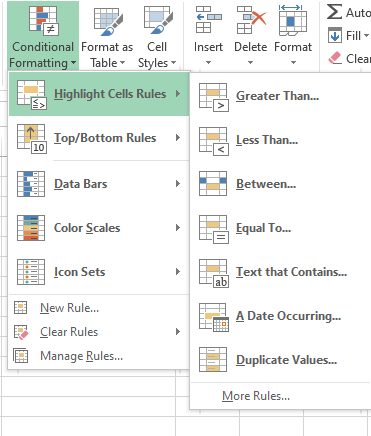Conditional formatting -> Highlight cell rules

For example, if we take the data on the average temperatures experienced month-wise (in F) and if we want to highlight the cells having temperature greater than 50 F (basically we want to visualize on the months having average temperature greater than 50 F), then we can use conditional formatting.

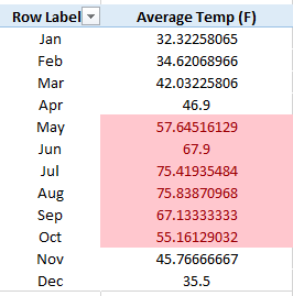All the months having temperature > 50 F

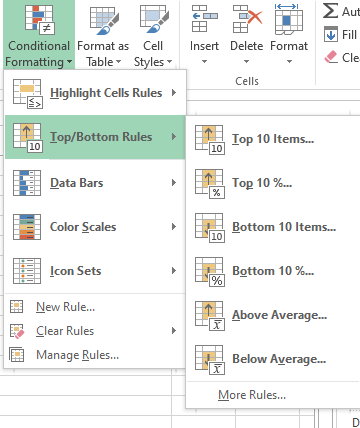
• Secondly, we can highlight the cells that are the top 10 items or the bottom 10 items or occur in the top 10% or bottom 10% of that particular column.

2. Data bars

It is also a great way to visualize relative values. Given below is the same example of average temperature displayed month-wise having the visualization of data bars. 

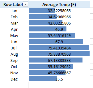We see that August has the maximum average temperature

We can also edit this formatting rule by going to the Manage rules option and then select the option of “Show only data bar” if we want only the data bars to be displayed and not the numbers. 

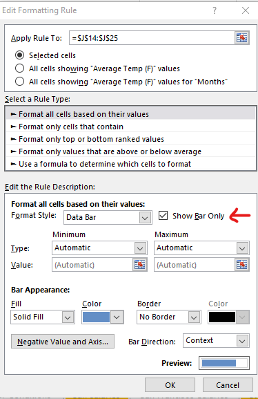
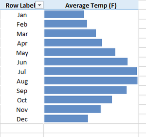Here only the data bars are shown and not the numbers. 

3. Color scales

A great way to create some heat maps for our data. So we will take the same example of displaying month-wise average temperatures. In this formatting, we will use a Red – White – Blue color scale in which maximum temperatures will be colored red and minimum will be colored blue. 

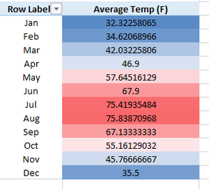So we can see that August was the hottest month and January was the coolest one. 

4. Icon sets

In this type of formatting, we use directional arrows, shapes, and various indicators to visualize our data. 

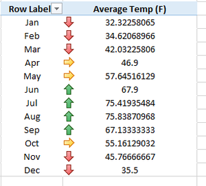We use green arrow for values > 67 and red arrow for values < 47.

5. Formula-based rules

We can also create our own rule and apply conditional formatting to them. 

• These were basically the 5 types of conditional formats that we can use to visualize our data in a more convenient and simpler way.
• If we want to clear any rule or edit any rule, we can simply go to the option of Clear rules and Manage rules respectively. We can clear any rule that we applied or edit it according to our choice.

Formula Based Rules

Methods to Apply Conditional Formatting to Pivot Table Cells

There are two methods to apply conditional formatting that make sure conditional formatting works even when there is new data in the backend.

How to Apply Conditional Formatting Using Pivot Table Formatting Icon

This Technique harnesses the power of the Pivot Table Formatting Options icon, which becomes available immediately after you’ve implemented conditional formatting within a pivot table.

Given below is the data set. (First Create a Pivot Table)

Pivot table

To employ this method, follow the below steps:

Step 1: Select the Data on which you want to apply conditional formatting.

Step 2: Go to Home and select Conditional Formatting.

Step 3: In conditional Formatting choose Top/Bottom Rules -> Above Average.

Step 4: Now specify the Format.

Specify the Format

Step 5: Click OK.

When you follow the above steps, it applies the conditional formatting on the data set. On the bottom right of the data set, you can see the Formatting Options icon.

Select the Icon

Click on the Icon. It will show following options in a drop down:

• Selected Cells
• All Cells Showing “Sum of Sales Amount”
• All cells Showing “Sum of Sales Amount” values for Name and Product.

Select the last option, So when you add any data in teh back end and refresh the Pivot Table, the additional data would automatically be covered by conditional formatting.

When working with conditional formatting in a pivot table, it’s essential to grasp the significance of three available options, each influencing how your formatting is applied:

Selected Cells:

This Stands as the default choice where conditional formatting solely impacts the cells you manually select. It’s ideal for focusing formatting efforts on specific areas of your Pivot Table, tailored to your immediate requirements.

All Cells Showing “Sum of Sales Amount” Values:

With this option, the conditional formatting encompasses all cells displaying the “Sum of Sales Amount” values. Yet, it’s vital to note a caveat- this approach extends to the Grand total values as well, affecting them with the same formatting.

All Cells Showing “Sum of Sales Amount” Values for Name and Product

Consider the most adept choice in this context, this option delivers comprehensive formatting while sidestepping the Grand Total dilemma. By applying conditional formatting to all values( excluding grand totals), it hones in on the combination of “Name” and “Product”. This strategic approach remains resilient even when additional data is introduced, seamlessly accommodating changes without intervention.

How to Apply Conditional Formatting Using Conditional Formatting Rules Manager

There is an alternative route to applying conditional formatting in Pivot tables using the Conditional Formatting rules manager Dialog Box. This method proves particularly valuable when you’ve already implemented conditional formatting and now seek to modify the existing rules:

Follow the steps to know how to execute this approach:

Step 1: Select the data where you wish to implement conditional formatting within the Pivot table.

Step 2: Naviagte to the “Home” tab, locate the “Conditional Formatting” option, and click over “Top/Bottom Rules”.

Step 3: From the dropdown menu, choose “Above Average”. This initiates the application of conditional formatting.

Step 4: Define the desired format.

Step 5: Click OK.

Step 6: Go back to the “Home” Tab, find “Condiitonal formatting,” and select , “Manage Rules”.

Step 7: In the ensuing “Conditional formatting Rules Manager” , pinpoint the rule you wish to modify, and select the “Edit Rule” button.

Step 8: Within the ‘”Edit Rule” dialog box, you ‘ll encounter the same trio of options:

Selected Cells

All cells showing “Sum of Sales Amount” Values.

All cells showing “Sum of Sales Amount” values for Name and Product.

Select the Last option and click OK.

Note: This will apply the conditional formatting to all the cells for ‘Name’ and ‘Product’ fields. Even if you change the backend data, the conditional formatting would be functional.

FAQs on Conditional Formatting in Pivot Table

What is Conditional Formatting in a Pivot Table?

Conditional Formatting in a Pivot table involves applying specific formatting styles, such as font color, background color, and cell borders, to cell based on predefined conditions. This helps highlight patterns, trends, and significant data points within the Pivot Table.

How to apply conditional formatting to a Pivot Table?

Follow the below steps to apply conditional formatting to a Pivot Table:

Step 1: Select the cells

Step 2: Go to Home tab and select Conditional Formatting. You can see a few choices- “Highlighting Cells Rules” or “Top/Bottom RUles”.

Step 3: Specify the format.

Where we can use Conditional formatting in Pivot table?

Conditional formatting is valuable for scenarios like:

• Identifying top or bottom values within categories.
• Highlighting values that exceed a certain threshold.
• Emphasizing variations in data through color scales.
• Spotting outliers or anomalies in the data.

How to modify or remove conditional formatting rules from a Pivot Table?

Follow the steps to modify or conditional formatting rules:

Step 1: Select the cells that you want to change the Special Formatting.

Step 2: Go to Home-> Conditional Formatting-> Manage Rules.

Step 3: In the “Conditional Formatting Rules Manager”, you can edit to even get rid of rules that are no longer needed.