How to Change Date Format in Excel

You know that Excel is one of the best spreadsheets you can work on. Excel is the first preference of many users to create an impressive data set. Have you tried filling in the Date on the sheet? Date with the data is a common practice done by users in Excel to get information timeline. To help organize data in an Excel worksheet, we will discuss four easy yet effective ways to change the date format in Excel.

What is the Date Format in Excel?

In Excel, a date is displayed depending on the user’s chosen format. You may choose from the different formats available in your Excel worksheet, or you can even create a customized date format per your requirements. The default date format is usually shown in your system’s ‘Control Panel.’ However, you can even change these default settings if necessary.

Change Date Format in Excel

When you input a date in Microsoft Excel, the program will format it according to the default date settings. For example, if you want to enter the date April 14, 2024, the date could appear in either long date format, or short date format, as 14-Apr, April 14, 2024, 14 April, or 04/14/2024, all depending on your settings. You may find that if you change a cell’s formatting to “Standard,” your date becomes stored as integers. For example, April 14, 2024, would become 47451, because Excel bases date formatting off of January 1, 1900. Each of these options are way to format dates in Excel. To help with organizing data in Excel, learn about how to change the date format in Excel.

How To Change Formatting of Date in Excel

You can change the date format using this method’s “Custom” option.

Follow the steps underneath:

Step 1: Select The Cell Range

Select the cell range.

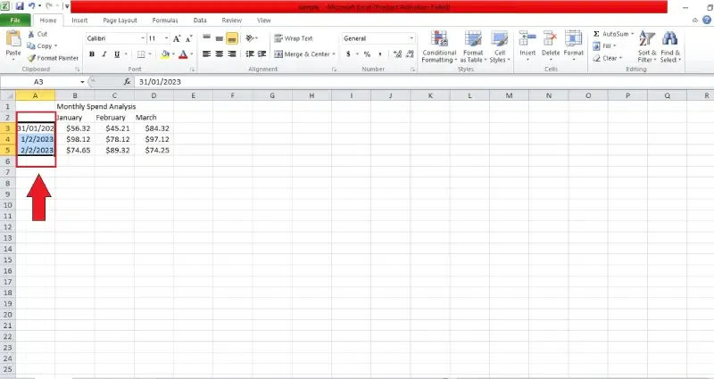
Select the cell range

Step 2: Go To Format Cells

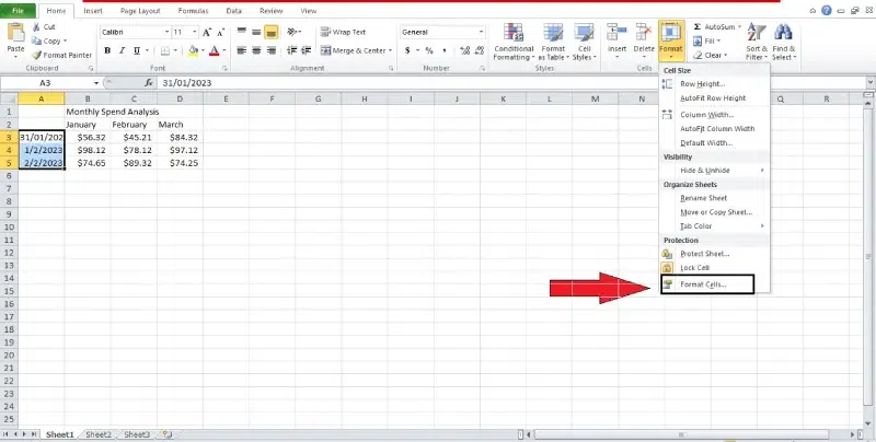
Next, you must go to the Home tab and then the Cell group. Then, click on the drop-down option showing format, and after that, choose the option showing Format Cells.

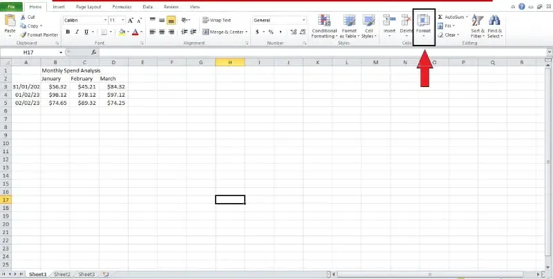
go to the Home tab and then the Cell group

Step 3: Choose Type

This is the third step, where you must select the Number bar from the Format Cells window. Next, go to the Category: group on the right side. Then, go to the option Type: group on the right side, and click on the option dd-mmmm-yyyy.

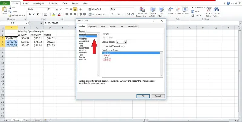
Select the Number bar from the Format Cells window

Step 4: Click OK

Lastly, click on OK and get your desired result.

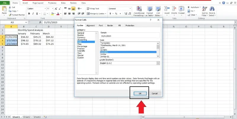
Click OK

How To Convert Date Formats to Other Locales

Suppose your worksheet shows dates in the US format, like mm-dd-yyyy. Now, if you want to change the formatting of the Date to the UK formatting rule, then here are the steps:

Step 1: Select the Data Range

First, you must select the date range on your Excel worksheet.

Select the Data Range

Step 2: Format Cells

After that, just hit the keys Ctrl + 1 to open the Format Cells dialogue box.

Format Cells dialogue box

Step 3: Select a Format from the Type list

This is the third step, where you must select a date format shown in the Type list.

Select a format from the Type list

Step 4: Change Format and Click Ok

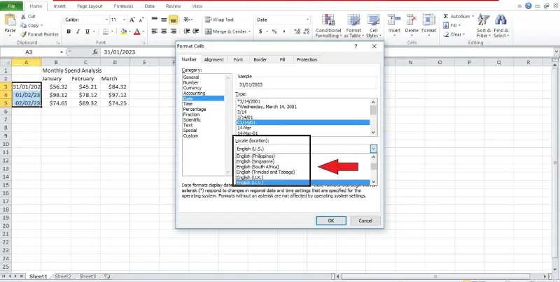
Now, click on the Locale drop-down menu below the Type list and select English (UK). Click OK button.

Select English (UK)

How To Change Date Format in Excel by Using Power Query

If you are trying to import a large database with inconsistent date formatting, use Power Query to get standard date formatting in your worksheet. In that case, you must use an effective tool called Power Query and follow these steps:

1. In this first step, click on the Add Column tab and then choose the Custom Column button.

2. Type a column name in the New column name field on the Custom Column wizard.

3.Inside the Custom column formula field, you have to enter the following formula:

=DateTime. To Text([DoJ], “dd-MM-yyyy”)

4.Now, click on the OK option to apply the formula.

5.Finally, you will see a new column in the Power Query tool with the date format you created. Then, delete the unnecessary date columns.

Note:

1. You must change the date system if negative numbers appear as dates.

2. Always ensure the cell is wide enough to fit the entire Date.

Tips for Displaying Dates in Excel

There are two ways to enter dates in cells: formulas for dynamic dates that compute the current Date or time interval or static dates that remain constant.

• If you want to add a date in multiple cells, then select the cell range, enter the formula, and press Ctrl+Enter to input the value in all of the selected cells.
• Mark a point that setting the Date & Time requires a change in the number formatting of the Date.
• The escape button helps you to restore the previous changees.

Suppose you’re looking for different Date functions to utilize in your formulae. In that case, you can also find them in the Date & Time menu on the formulae tab of the Ribbon.

Default Date Format in Excel

The Date that you enter in the Excel workbook is automatically reflected in the format of the month first, then the day, and then the year. The default date format in the Excel workbook is mm/dd/yyyy format.

Dates entered into cells in Excel typically use the slash as their default delimiter between the day, month, and year.

Plus, this is constant regardless of whether you use dashes or not when writing your Date. Excel changes the dashes to slashes immediately.

How to Change the Default Date and Time Formats in Excel

Follow the steps mentioned below to change the default date and time formats in Excel:

Select the cell range in your Excel workbook that you want to format and press Control+1.

Go to the Cells option in the Home tab and click on the Format Cells tab box.

From the drop-down menu of the Home tab, select the “Number” option. Select “date” from the options mentioned on the screen.

How to Quickly Apply Default Date and Time Formatting in Excel

Step 1: Select the cell and Enter the formula

Click on the cell that consists of the Date or enter the Date in a blank cell. Enter the CTRL+SHIFT+# or CTRL+SHIFT+@ formula in the cell.

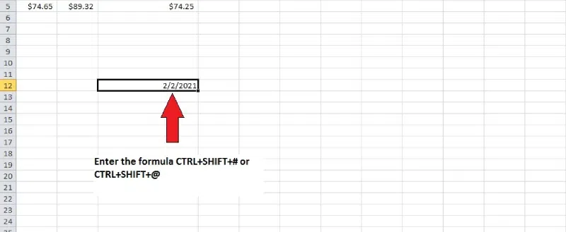
Enter the CTRL+SHIFT+# or CTRL+SHIFT+@ formula

How to Change the Default Time Format

Step 1: Select the Cell

Click on the cell that consists of Time or enter the Time in a blank cell.

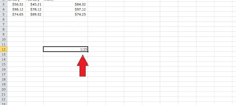
Select the cell

Step 2: Go to the Home tab

In the Home tab, click the Number group.

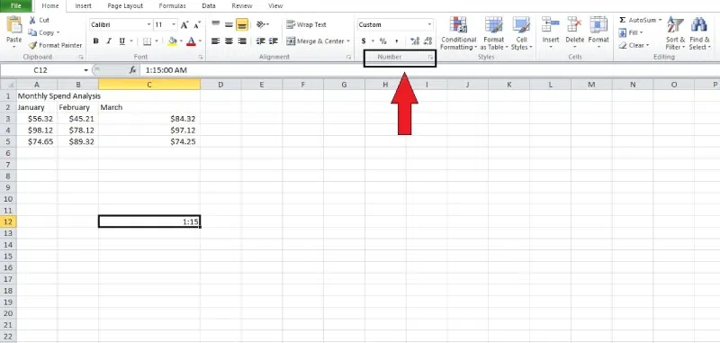
Go to the Home tab

Step 3: Select Time

Choose Time from the Number Format drop-down list.

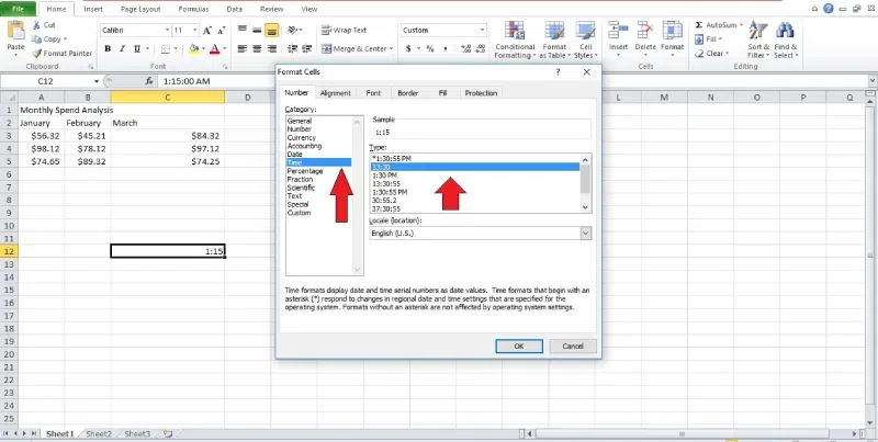
Select Time

Conclusion

Though changing the date format is a small task, singing it enhances the data presentation in your Excel worksheet. It is not only simple to share but also easy to understand. This article mentions all four methods of changing the date format in your Excel workbook. Follow each step in the sequence to make your datasheet presentation visually appealing. You can choose any method; the result will always be the same without any hustle.

FAQ’s on How to Change Date Format in Excel

Why is the date format in my Excel Not changing?

If the date format in your Excel worksheet is not changing, then your dates may be formatted as text. Hence, you have to convert them to the date format first.

How do I change the date format in Excel to UK?

1. Open an Excel spreadsheet on your desktop.
2. Select the file and click “Options.”
3. The “Regional Format settings” tab opens. Click on the drop-down box and tap on the region.
4. Tap on “Change”.

How do I convert text to Date in Excel?

1. Assume your Date is in cell A1.
2. In a different cell, type =DATEVALUE(A1).
3. Hit Enter to apply the formula.
4. Right-click the cell with the formula.
5. Select “Format Cells” from the menu.
6. In the Number tab, choose Date from the list.
7. Confirm by clicking OK.

How do I convert a date to a month in Excel?

You can convert a date to a month in Excel using the MONTH function

Suppose your Date is in cell A1.

In another cell, type =MONTH(A1).

Press Enter.

It will return the month number (1 for January, 2 for February, etc.) of the Date in cell A1.

If you want the month name instead of the month number, you can use the TEXT function in combination with the MONTH function:

Suppose your Date is in cell A1.

In another cell, type =TEXT(A1, “mmmm”).

Press Enter.