Cycle Generative Adversarial Network (CycleGAN)

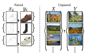
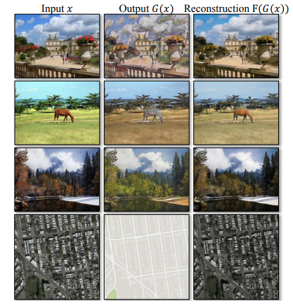
GANs was proposed by Ian Goodfellow . Cycle GAN is used to transfer characteristic of one image to another or can map the distribution of images to another. In CycleGAN we treat the problem as an image reconstruction problem. We first take an image input (x) and using the generator G to convert into the reconstructed image. Then we reverse this process from reconstructed image to original image using a generator F. Then we calculate the mean squared error loss between real and reconstructed image. The most important feature of this cycle_GAN is that it can do this image translation on an unpaired image where there is no relation exists between the input image and output image. 

Architecture 

Like all the adversarial network CycleGAN also has two parts Generator and Discriminator, the job of generator to produce the samples from the desired distribution and the job of discriminator is to figure out the sample is from actual distribution (real) or from the one that are generated by generator (fake).

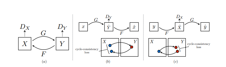
The CycleGAN architecture is different from other GANs in a way that it contains 2 mapping function (G and F) that acts as generators and their corresponding Discriminators (Dx and Dy): The generator mapping functions are as follows:

where X is the input image distribution and Y is the desired output distribution (such as Van Gogh styles) . The discriminator corresponding to these are:

Dx :  distinguish G(X)(Generated Output) from Y (real Output )

Dy : distinguish F(Y)(Generated Inverse Output) from X (Input distribution)

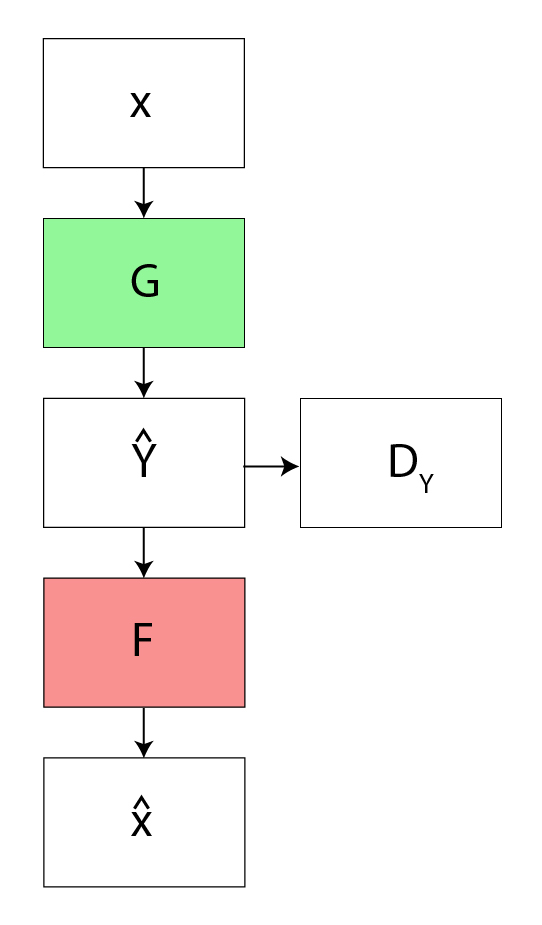
To further regularize the mappings, the authors used two more loss function in addition to adversarial loss . The forward cycle consistency loss and the backward cycle consistency loss . The forward cycle consistency loss refines the cycle : 

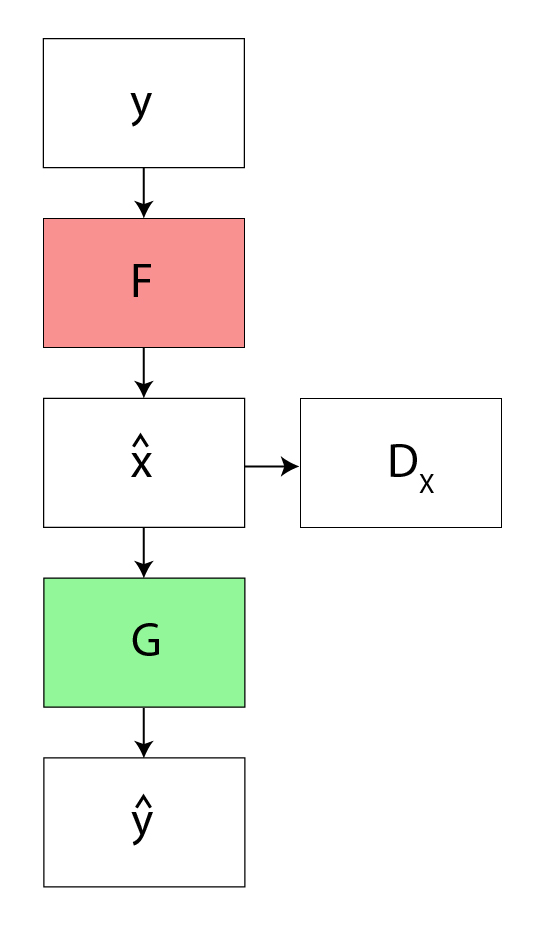
The backward cycle consistency loss refines the cycle:

Generator Architecture:

Each CycleGAN generator has three sections:

• Encoder
• Transformer
• Decoder

The input image is passed into the encoder. The encoder extracts features from the input image by using Convolutions and compressed the representation of image but increase the number of channels. The encoder consists of 3 convolution that reduces the representation by 1/4 th of actual image size. Consider an image of size (256, 256, 3) which we input into the encoder, the output of encoder will be (64, 64, 256).

Then the output of encoder after activation function is applied is passed into the transformer. The transformer contains 6 or 9 residual blocks based on the size of input. The output of transformer is then passed into the decoder which uses 2 -deconvolution block of fraction strides to increase the size of representation to original size.

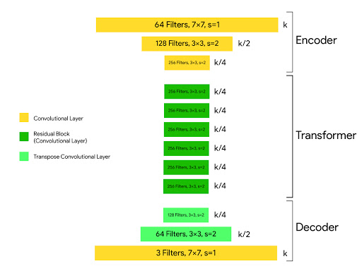
The architecture of generator is:

c7s1-64, d128, d256, R256, R256, R256,

R256, R256, R256, u128, u64, c7s1-3 

where c7s1-k denote a 7×7 Convolution-InstanceNorm-ReLU layer with k filters and stride 1. dk denotes a 3 × 3 Convolution-InstanceNorm-ReLU layer with k filters and stride 2. Rk denotes a residual block that contains two 3 × 3 convolution layers with the same number of filters on both layer. uk denotes a 3 × 3 fractional-strides-Convolution-InstanceNorm-ReLU layer with k filters and stride 1/2 (i.e deconvolution operation).

Discriminator Architecture:

In discriminator the authors use PatchGAN discriminator. The difference between a PatchGAN and regular GAN discriminator is that rather the regular GAN maps from a 256×256 image to a single scalar output, which signifies “real” or “fake”, whereas the PatchGAN maps from 256×256 to an NxN (here 70×70) array of outputs X, where each X_ij signifies whether the patch ij in the image is real or fake. 

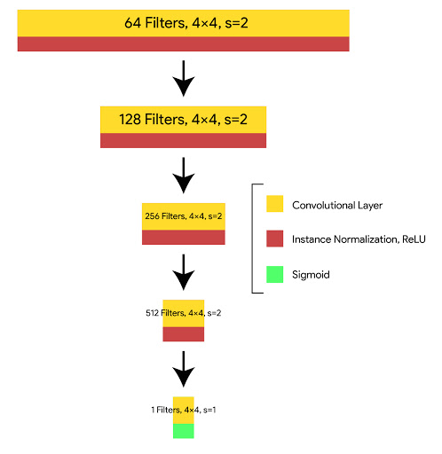
The architecture of discriminator is : 

C64-C128-C256-C512

where Ck is 4×4 convolution-InstanceNorm-LeakyReLU layer with k filters and stride 2. We don’t apply InstanceNorm on the first layer (C64). After the last layer, we apply convolution operation to produce a 1×1 output.

Cost Function:

• Adversarial Loss:  We apply adversarial loss to both our mappings of generators and discriminators. This adversary loss is written as :

• Cycle Consistency Loss: Given a random set of images adversarial network can map the set of input image to random permutation of images in the output domain which may induce the output distribution similar to target distribution. Thus adversarial mapping cannot guarantee the input x_i  to y_i . For this to happen the author proposed that process should be cycle-consistent. This loss function used in Cycle GAN to measure the error rate of  inverse mapping G(x) -> F(G(x)). The behavior induced by this loss function cause closely matching the real input (x) and F(G(x))

The Cost function we used is the sum of adversarial loss and cyclic consistent loss:

and our aim is :

Applications:

• Collection Style Transfer:  The authors trained the model on landscape photographs downloaded from Flickr and WikiArt. Unlike other works on neural style transfer, CycleGAN learns to mimic the style of an entire collection of artworks, rather than transferring the style of a single selected piece of art. Therefore it can generate different  styles such as : Van Gogh, Cezanne, Monet, and Ukiyo-e .

Style Transfer Results

Comparison of different Style Transfer Results

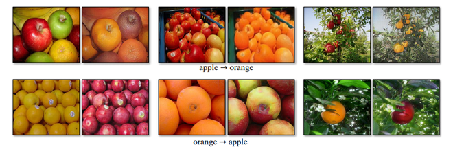
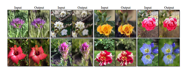
• Object Transformation: CycleGAN can transform object from one ImageNet class to another such as: Zebra to Horses and vice-versa, Apples to Oranges and vice versa etc.
  • Apple <—> Oranges:

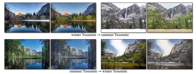
• Season Transfer: CycleGAN can also transfer images from Winter Season to Summer season and vice-versa. For this the model is trained on 854 winter photos and 1273 summer photos of Yosemite from Flickr.

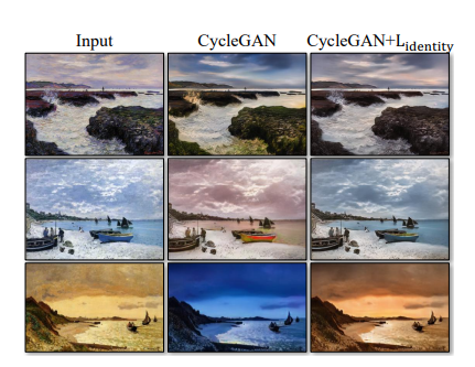
• Photo Generation from Painting: CycleGAN can also be used to transform photo from paintings and vice-versa. However to improve this transformation., the authors also introduced an additional loss called Identity loss. This loss can be defined as :

• Photo enhancement : CycleGAN can also be used for photo enhancement. For this the model takes images from two categories which are captured from smartphone camera (usually have deep Depth of Field due to low aperture ) to DSLR (which have lower depth of Field). For this task the model transforms images from smartphone to DSLR quality images.

Evaluation Metrics:

• AMT perceptual Studies : For the map?aerial photo task, the authors run “real vs fake” perceptual studies on Amazon Mechanical Turk (AMT) to assess the realism of our outputs. . Participants were shown a sequence of pairs of images, one a real photo or map and one fake (generated by our algorithm or a baseline), and asked to click on the image they thought was real.
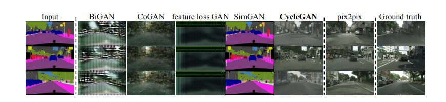
• FCN Scores: For Cityscapes labels?photo dataset the authors FCN score . The FCN predicts a label map for a generated photo. This label map can then be compared against the input ground truth labels using standard semantic segmentation metrics. Here the standard segmentation metrics that are used in Cityscapes dataset such as per-pixel accuracy, per class IoU and mean class IoU.

Results:

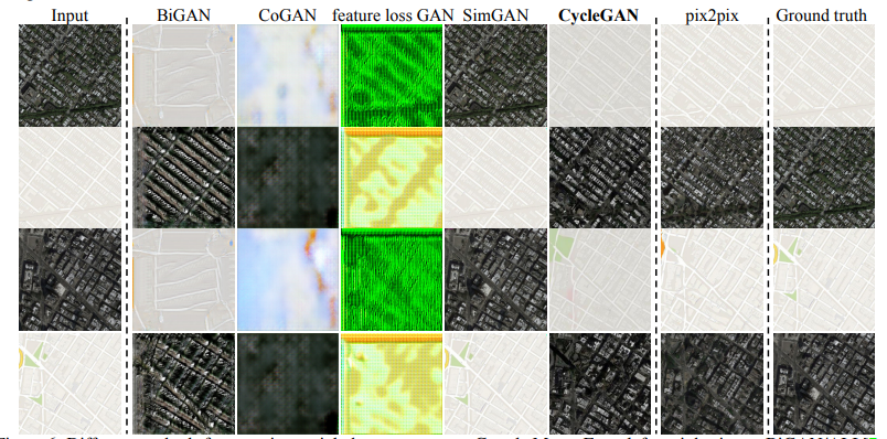
• For map?aerial task, the results on AMT “real vs fake” test are as follows:

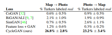
In this task the authors scrap data from Google Maps and google Earth and evaluated on different GANs method and compared to Ground Truth.

Classification Performance for different metrics

Some of the results from Cityscapes dataset are as follows

Drawbacks and Limitations :

• CycleGAN can be useful when we need to perform color or texture transformation, however when applied to perform geometrical transformation, CycleGAN does not perform very well. This is because of the generator architecture which is trained to perform appearance changes in the image.

Failure Cases of Cycle GAN

References:

• Unpaired Image-to-Image Translation using Cycle-Consistent Adversarial Networks