Creating Hybrid Images Using OpenCV Library | Python

Hybrid image, or “multi-scale image”, is an exciting concept in computer vision. They are created by blending one image’s high-frequency components with another’s low-frequency components. The result is an image that appears as one when viewed from a distance but shows a different image when viewed up close.

The following are the steps for creating a hybrid image of two photos using OpenCV library in python:

1. Find the fourier transformation of both the images and apply zero component center shifting.
2. Extract the low frequency component and high frequency component from images.
3. Get the image of low frequency and high frequency component using Inverse Fourier transformation.
4. Combine the spatial domain of the low-pass filtered image and high-pass filtered image by adding their magnitudes elementwise.

Consider two images as shown below for the implementation:

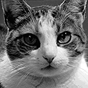
Cat.png

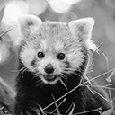
Panda.png

Implementation: Creating Hybrid Images Using OpenCV Library

Import the necessary libraries

The code imports libraries for image processing including OpenCV (cv2), PIL (Image), NumPy, and matplotlib. It also imports the square root (sqrt) and exponential (exp) functions from the math module.

Python3

import cv2
from PIL import Image
import numpy as np
import matplotlib.pyplot as plt
from math import sqrt, exp

Custom Function for Plotting Image

The code defines two custom functions:

1. plot_figure: Plots a grid of images with corresponding titles, allowing customization of the figure size, number of rows, and columns.
2. distance: Calculates the Euclidean distance between two points given as tuples of (x, y) coordinates.

Python3

#Custom Function for Image Plotting
def plot_figure(images: list, titles: list, rows: int, columns: int, fig_width=15, fig_height=7):
    fig = plt.figure(figsize=(fig_width, fig_height))
    count = 1
    for image, title in zip(images, titles):
        fig.add_subplot(rows, columns, count)
        count += 1
        plt.imshow(image, 'gray')
        plt.axis('off')
        plt.title(title)
 

#Custom Function to get Euclidean Distance
def distance(point1, point2):
    return sqrt((point1[0] - point2[0]) ** 2 + (point1[1] - point2[1]) ** 2)

Extracting Low Frequency Component

The function creates a Gaussian low-pass filter to extract low-frequency components. The `D0` parameter determines the cutoff frequency of the filter, controlling which frequencies are considered low. It iterates over each pixel and calculates its value based on its distance from the center of the filter and the cutoff frequency `D0`. Pixels closer to the center and with lower frequencies will have higher values, emphasizing low-frequency content.

Python3

#Function to get low frequency component
#D0 is cutoff frequency
def gaussianLP(D0, imgShape):
    base = np.zeros(imgShape[:2])
    rows, cols = imgShape[:2]
    center = (rows/2, cols/2)
    for i in range(rows):
        for j in range(cols):
            base[i, j] = np.exp(-distance((i, j), center)**2 / (2 * D0**2))
    return base

Extracting High Frequency Component

The function creates a Gaussian high-pass filter to extract high-frequency components. The `D0` parameter determines the cutoff frequency of the filter, controlling which frequencies are considered high. It iterates over each pixel and calculates its value based on its distance from the center of the filter and the cutoff frequency `D0`. Pixels farther from the center and with higher frequencies will have higher values, emphasizing high-frequency content.

Python3

#Function to get high frequency component
#D0 is cutoff frequency
def gaussianHP(D0, imgShape):
    base = np.zeros(imgShape[:2])
    rows, cols = imgShape[:2]
    center = (rows/2, cols/2)
    for i in range(rows):
        for j in range(cols):
            base[i, j] = 1 - np.exp(-distance((i, j), center)**2 / (2 * D0**2))
    return base

Hybrid Image Function

The function returns a hybrid image from two input images. It separates the high and low-frequency components of each image using Fourier transforms and Gaussian filters. The low-frequency components of one image are combined with the high-frequency components of the other image. The `D0` parameter controls the amount of high-frequency information retained, affecting the clarity of the close-up image.

Python3

#Function to generate hybrid image
#D0 is cutoff frequency
def hybrid_images(image1, image2, D0 = 50):
    original1 = np.fft.fft2(image1)                          #Get the fourier of image1
    center1 = np.fft.fftshift(original1)                     #Apply Centre shifting
    LowPassCenter = center1 * gaussianLP(D0, image1.shape)   #Extract low frequency component
    LowPass = np.fft.ifftshift(LowPassCenter)                 
    inv_LowPass = np.fft.ifft2(LowPass)                         #Get image using Inverse FFT

    original2 = np.fft.fft2(image2)
    center2 = np.fft.fftshift(original2)
    HighPassCenter = center2 * gaussianHP(D0, image2.shape)  #Extract high frequency component
    HighPass = np.fft.ifftshift(HighPassCenter)
    inv_HighPass = np.fft.ifft2(HighPass)
    hybrid = np.abs(inv_LowPass) + np.abs(inv_HighPass)      #Generate the hybrid image
    return hybrid

Main Function

Python3

# Load images
# Make sure to choose the same image format for both images (Ex- .png)
A = cv2.imread('/content/cat.png',cv2.IMREAD_COLOR) # high picture
B = cv2.imread('/content/panda.png',cv2.IMREAD_COLOR) # low picture

# Convert both images to Grayscale to avoid any Color Channel Issue
A_grayscale = cv2.cvtColor(A, cv2.COLOR_BGR2GRAY)
B_grayscale = cv2.cvtColor(B, cv2.COLOR_BGR2GRAY)

# Resize both images to 128x128 to avoid different image size issue
A_resized = cv2.resize(A_grayscale, (128, 128))
B_resized = cv2.resize(B_grayscale, (128, 128))

result = hybrid_images(A_resized,B_resized,1)

plot_figure([A,B,result], ['A','B','Hybrid Image'],1,3)

Output: