COVID-19 Peak Prediction using Logistic Function
Last Updated :
05 Aug, 2021
Making fast and accurate decisions are vital these days and especially now when the world is facing such a phenomenon as COVID-19, therefore, counting on current as well as projected information is decisive for this process.
In this matter, we have applied a model in which is possible to observe the peak in specific country cases, using current statistical information, hoping it can be used as foundation support to take action in this scenario. To accomplish this objective, Non-linear regression has been applied to the model, using a logistic function. This process consists of:
- Data Cleaning
- Choosing the most suitable equation which can be graphically adapted to the data, in this case, Logistic Function (Sigmoid)
- Database Normalization
- Fitting of the model to our dataset using “curve_fit” process, obtaining new reference beta.
- Model evaluation
Dataset is public, and it is available at Data.europa.eu following this link: DATASET
Data Cleaning: The data available has been originally labelled. We were able to identify two countries which did not mention geographical location, this information was added however it wouldn´t contribute to the model significantly. A new column is added to the dataset named “n-day” to show the consecutive number of days.
Code: Importing Libraries
Python3
import pandas as pd
import numpy as np
import matplotlib.pyplot as plt % matplotlib inline
from sklearn.metrics import r2_score
|
Code: Using data
Python3
df = pd.read_excel("C:/BaseDato / COVID-19-310302020chi.xlsx")
df.head()
|
Output:

Code:
Python3
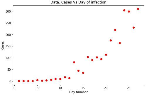
plt.figure(figsize =(8, 5))
x_data, y_data = (df["Nday"].values, df["cases"].values)
plt.plot(x_data, y_data, 'ro')
plt.title('Data: Cases Vs Day of infection')
plt.ylabel('Cases')
plt.xlabel('Day Number')
|
Output:
Code: Choosing the model
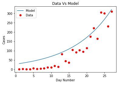
We apply logistic function, a specific case of sigmoid functions, considering that the original curve starts with slow growth remaining nearly flat for a time before increasing, eventually it could descend or maintain its growth in the way of an exponential curve.
The formula for the logistic function is:
Y = 1/(1+e^B1(X-B2))
Code: Construction of the model
Python3
def sigmoid(x, Beta_1, Beta_2):
y = 1 / (1 + np.exp(-Beta_1*(x-Beta_2)))
return y
beta_1 = 0.09
beta_2 = 305
Y_pred = sigmoid(x_data, beta_1, beta_2)
plt.plot(x_data, Y_pred * 15000000000000., label = "Model")
plt.plot(x_data, y_data, 'ro', label = "Data")
plt.title('Data Vs Model')
plt.legend(loc ='best')
plt.ylabel('Cases')
plt.xlabel('Day Number')
|
Output:
Data Normalization: Here, variables x and y are normalized assigning them a 0 to 1 range (depending on each case). So both can be interpreted in equal relevance.
Reference – information
Code:
Python3
xdata = x_data / max(x_data)
ydata = y_data / max(y_data)
|
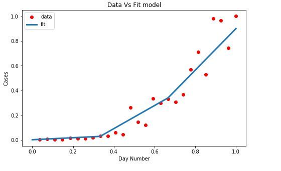
Model Fitting:
The objective is to obtain new B optimal parameters, to adjust the model to our data. We use “curve_fit” which uses non-linear least squares to fit the sigmoid function. Being “popt” our optimized parameters.
Code: Input
Python3
from scipy.optimize import curve_fit
popt, pcov = curve_fit(sigmoid, xdata, data)
print(" beta_1 = % f, beta_2 = % f" % (popt[0], popt[1]))
|
Output:
beta_1 = 9.833364, beta_2 = 0.777140
Code: New Beta values are applied to the model
Python3
x = np.linspace(0, 40, 4)
x = x / max(x)
plt.figure(figsize = (8, 5))
y = sigmoid(x, *popt)
plt.plot(xdata, ydata, 'ro', label ='data')
plt.plot(x, y, linewidth = 3.0, label ='fit')
plt.title("Data Vs Fit model")
plt.legend(loc ='best')
plt.ylabel('Cases')
plt.xlabel('Day Number')
plt.show()
|
Model Evaluation: The model is ready to be evaluated. The data is split in at 80:20, for training and testing respectively. The data is applied to the model obtaining the corresponding statistical means to evaluate the distance of the resulting data from the regression line.
Code: Input
Python3
L = np.random.rand(len(df)) < 0.8
train_x = xdata[L]
test_x = xdata[~L]
train_y = ydata[L]
test_y = ydata[~L]
popt, pcov = curve_fit(sigmoid, train_x, train_y)
y_predic = sigmoid(test_x, *popt)
print("Mean Absolute Error: %.2f" % np.mean(np.absolute(y_predic - test_y)))
print("Mean Square Error (MSE): %.2f" % np.mean(( test_y - y_predic)**2))
print("R2-score: %.2f" % r2_score(y_predic, test_y))
|
Output:
Mean Absolute Error: 0.06
Mean Square Error (MSE): 0.01
R2-score: 0.93
Share your thoughts in the comments
Please Login to comment...